Online RLadies

@SherlockpHolmes

The slides : https://bios221.stanford.edu/NetworkSlides.html

See Github repo: spholmes/GraphsTutorial

Install with:

devtools::install_github("spholmes/GraphsTutorial")

Introduction

In this worksheet, we will discuss how to visualize networks using the tidyverse.

We will be using the R package tidyverse, which includes ggplot() and related functions.

# load required library
library(tidyverse)

We use specialized packages for graphs based on the igraph package, the tidyverse compatible ones are ggnetwork and ggraph.

# load required library
library(igraph)
library(tidygraph)
library(ggnetwork)
library(ggraph)

We will use a package which is on BIOCONDUCTOR and not on CRAN, so you need to also install it using:

if (!requireNamespace("BiocManager", quietly = TRUE))
    install.packages("BiocManager")

BiocManager::install("phyloseq")

What is a graph ?

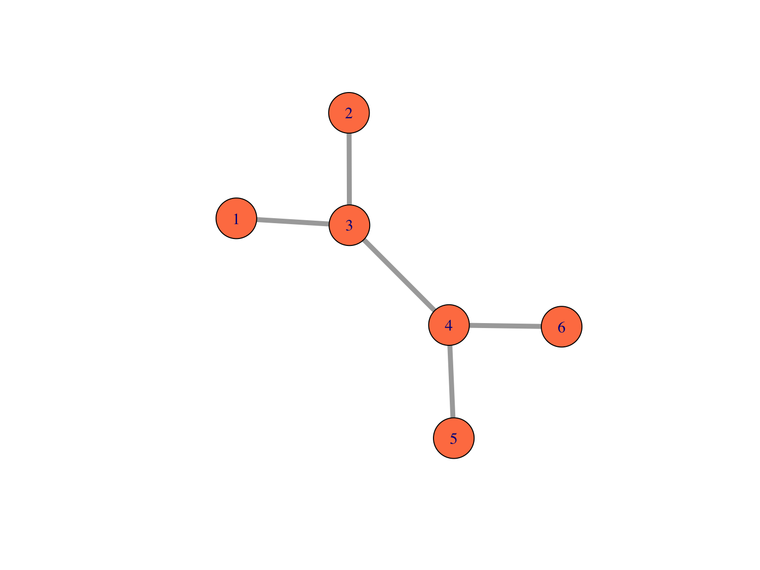
A small undirected graph with numbered nodes.

Here is the adjacency matrix of the small undirected graph represented below. We see that \(A\) is symmetric \(n \times n\) matrix of \(0\)’s and \(1\)’s.

A=as_adj(g1, sparse = FALSE)
A

##      [,1] [,2] [,3] [,4] [,5] [,6]
## [1,]    0    0    1    0    0    0
## [2,]    0    0    1    0    0    0
## [3,]    1    1    0    1    0    0
## [4,]    0    0    1    0    1    1
## [5,]    0    0    0    1    0    0
## [6,]    0    0    0    1    0    0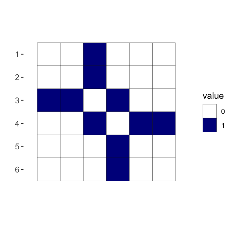

Here is how we plot a simple graph:

library("igraph")
edges1 = matrix(c(1,3,2,3,3,4,4,5,4,6), byrow = TRUE, ncol = 2)
g1 = graph_from_edgelist(edges1, directed = FALSE)
plot(g1, vertex.size = 25, edge.width = 5, vertex.color = "coral")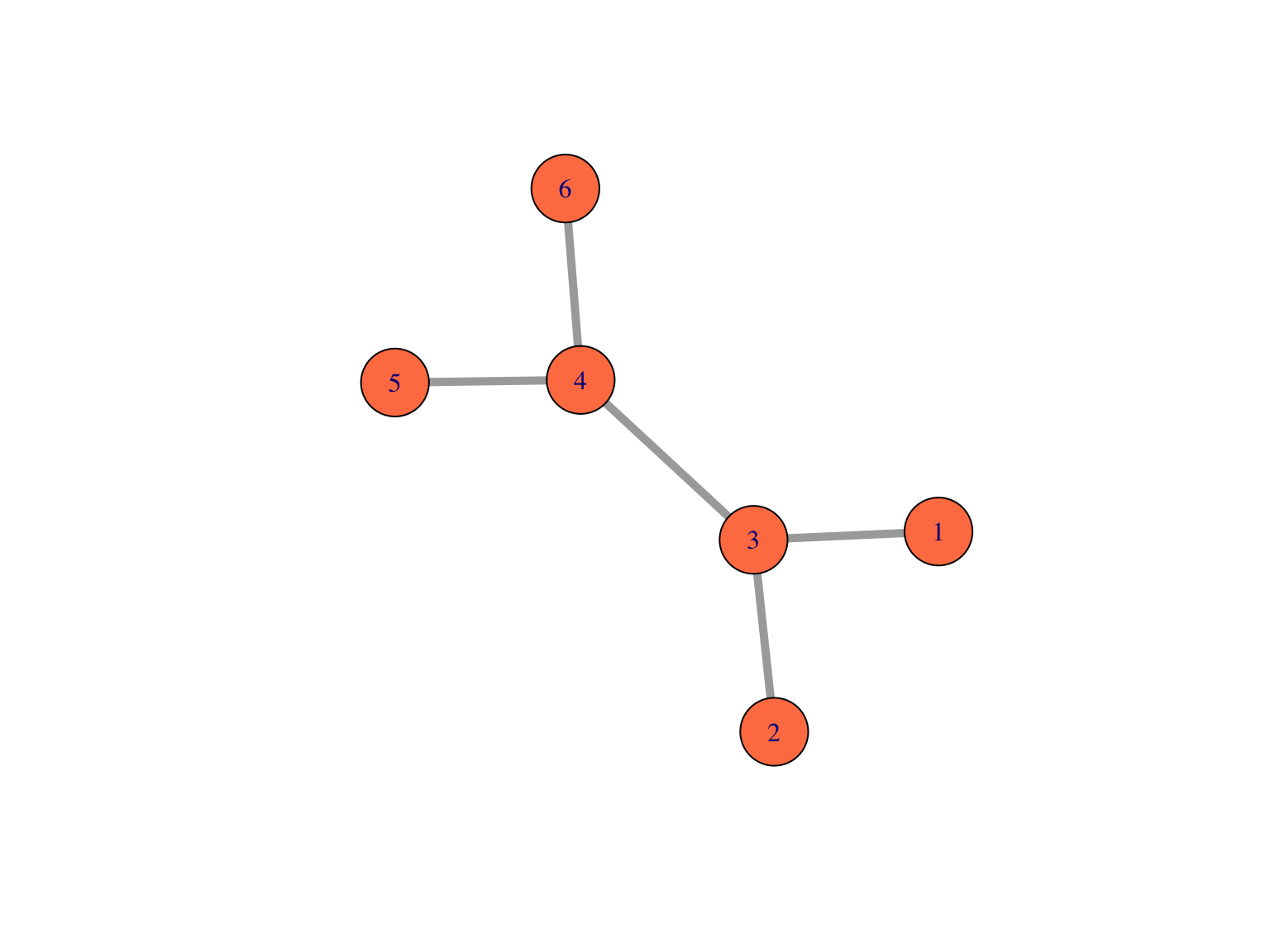

Modify the Code to change the color of the node labels

Now add two lines that label the nodes:

library("igraph")
edges1 = matrix(c(1,3,2,3,3,4,4,5,4,6), byrow = TRUE, ncol = 2)

Other ways to enter graph data

Can you think of an alternative way of reading the graph from an edge set dataframe (the code should be two or three lines) and then plotting it?

edges=_____
sg =  _____ 

## IGRAPH 38bd453 UN-- 7 6 -- 
## + attr: name (v/c)
## + edges from 38bd453 (vertex names):
## [1] 1--3 2--3 3--4 4--6 4--5 1--7

Elements of a simple graph:

plot(sg, vertex.size = 35, edge.width = 7, vertex.color = "purple",vertex.label.color="white")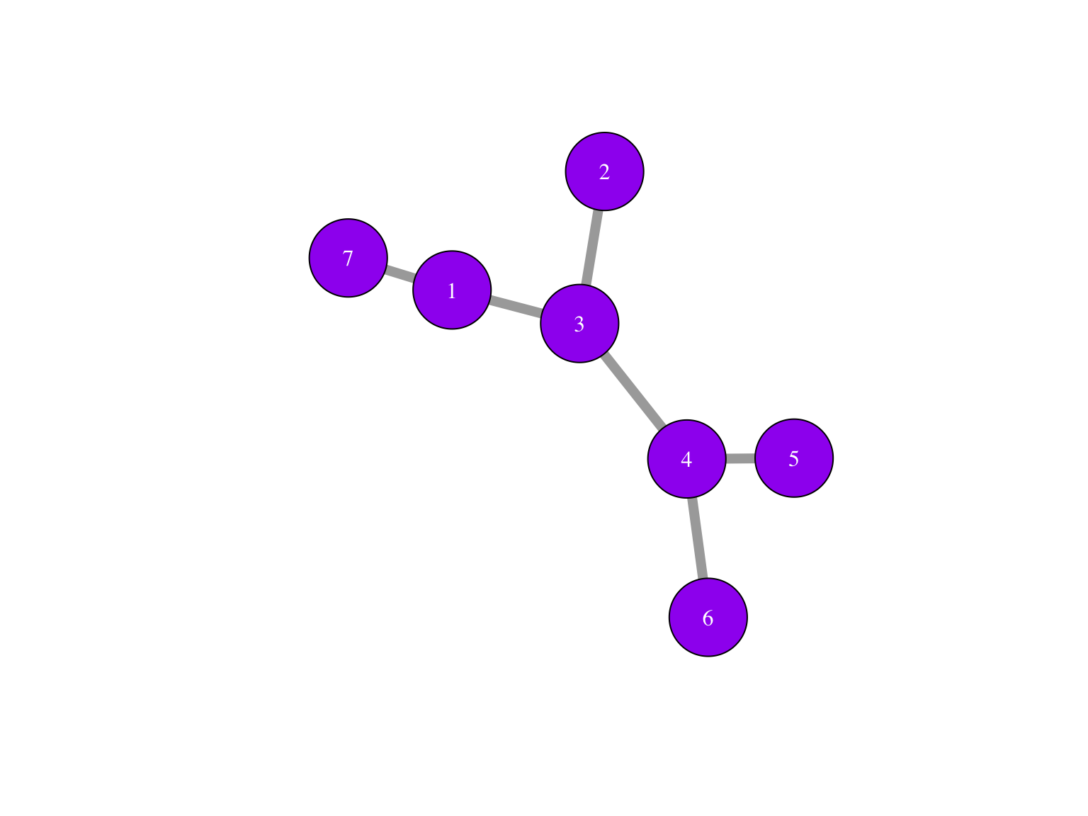

• The nodes or vertices which are the colored circles with numbers in them in the Figure.

• Edges or connections, the segments that join the nodes and which can be directed or not.

• Edge lengths, when not specified, we suppose they are all one and compute the distance between vertices on the graph as the number the edges traversed. On the other hand, in many situations we have meaningful edge lengths or strengths of connections between vertices that we can use both in the plots and analyses.

And a network?

• We call a weighted, directed graph a network. Networks have adjacency matrices \(A\) which are \(n\) by \(n\) matrices of positive numbers corresponding to the edge lengths.

• Edge and node attributes: optionally, each edge or each node can be mapped to further continuous or categorical variables.

Networks can be given to us in databases

As a starting example, the following data came from the STRING database, it is a chemokine network formatted as a txt file.

Starting with a txt file for instance

Look at the file linked here

We read the file in as a simple table for the time being.

chemodats =read.table("https://web.stanford.edu/class/bios221/data/small_chemokine.txt",header=TRUE) 

Making a graph from the list of nodes and edges

dim(chemodats)

## [1] 20 15

head(chemodats[,1:4])

##   node1  node2 node1_string_id node2_string_id
## 1 CXCR3   CCR7         1855969         1843829
## 2 ITGA4    EED         1858446         1845338
## 3 CXCR5 CXCL13         1847335         1847033
## 4   PF4  CXCR5         1847665         1847335
## 5  THBD    PF4         1856612         1847665
## 6 CCL19   CCR7         1849114         1843829

Question: What does each row of chemodats correspond to?

Our first function is graph_from_data_frame from the igraph package:

gr = graph_from_data_frame(chemodats[,c("node1", "node2")], directed = FALSE)
E(gr)$weight = 1
V(gr)$size = centralization.degree(gr)$res
saveRDS(gr,file="../gr.RDS")

We created an annotation variable for the nodes. This was computed a the centralization index of the nodes with regards to this graph (larger nodes are more central to the graph).

Now we have an igraph object, how would you plot it?

____(gr)

Question: What would you type in order to find out which are the default plotting parameters for this inherited plot of an igraph object?

_____

This plot function is the equivalent of a simple base R plot for gr which is an object of type igraph.

Creating a graph from distance data

The most common form of network that we create from data comes from some measure that we have available between the points that will be vertices of the graph. Suppose we are provided with a dist object from a distance computation between samples or nodes. There are several ways a graph can be constructed from this starting point.

Minimum spanning trees

library("igraph")
library("ggnetwork")
library("ggplot2")
pts = structure(c(0, 0, 1, 1, 1.5, 2, 0, 1, 1, 0, 0.5, 0.5),
                .Dim = c(6L,2L))
matxy = pts
distxy = stats::dist(matxy)
g = graph.adjacency(as.matrix(distxy), weighted = TRUE)
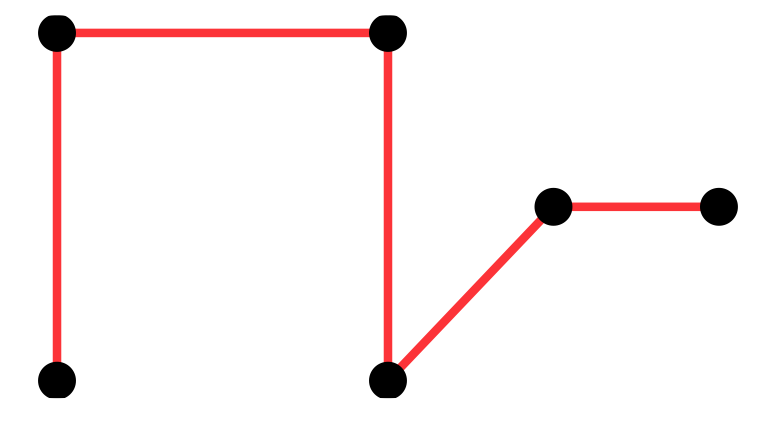
mst1 = igraph::mst(g)

A spanning tree is a tree that goes through all points at least once, the graph with red edges is such a tree.

The minimum spanning tree is the spanning tree with the shortest length.

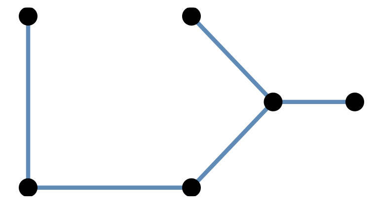
Minimum spanning trees (MST) are easy/cheap to compute and there are many different functions in R packages that provide them:

igraph::mst ape::mst ade4::mstree vegan::spantree spdep::mstree

Example: A graph created from DNA distance data

An example distance matrix was created between strains of HIV from different patients whose countries were recorded.

We can read in the DNA distance data that was provided.

Using ggnetwork and ape::mst

library(ggplot2)
library(igraph)
library(ggnetwork)
load(url("https://web.stanford.edu/class/bios221/data/dist2009c.RData"))
country09 = attr(dist2009c, "Label")
mstree2009 = ape::mst(dist2009c)
gr09 = graph.adjacency(mstree2009, mode = "undirected")
gg = ggnetwork(gr09, arrow.gap = 0, layout = layout_with_fr(gr09))
ggplot(gg, aes(x = x, y = y, xend = xend, yend = yend)) +
  geom_edges(color = "black", alpha = 0.5, curvature = 0.1) +
  geom_nodes(aes(color = name), size = 2) +  theme_blank() +
  geom_nodetext(aes(label = name), color = "black", size = 2.5) +
  theme(plot.margin = unit(c(0, 1, 1, 6), "cm"))+
   theme(legend.position = c(0, 0.14),
      legend.background = element_blank(),
      legend.text = element_text(size = 7))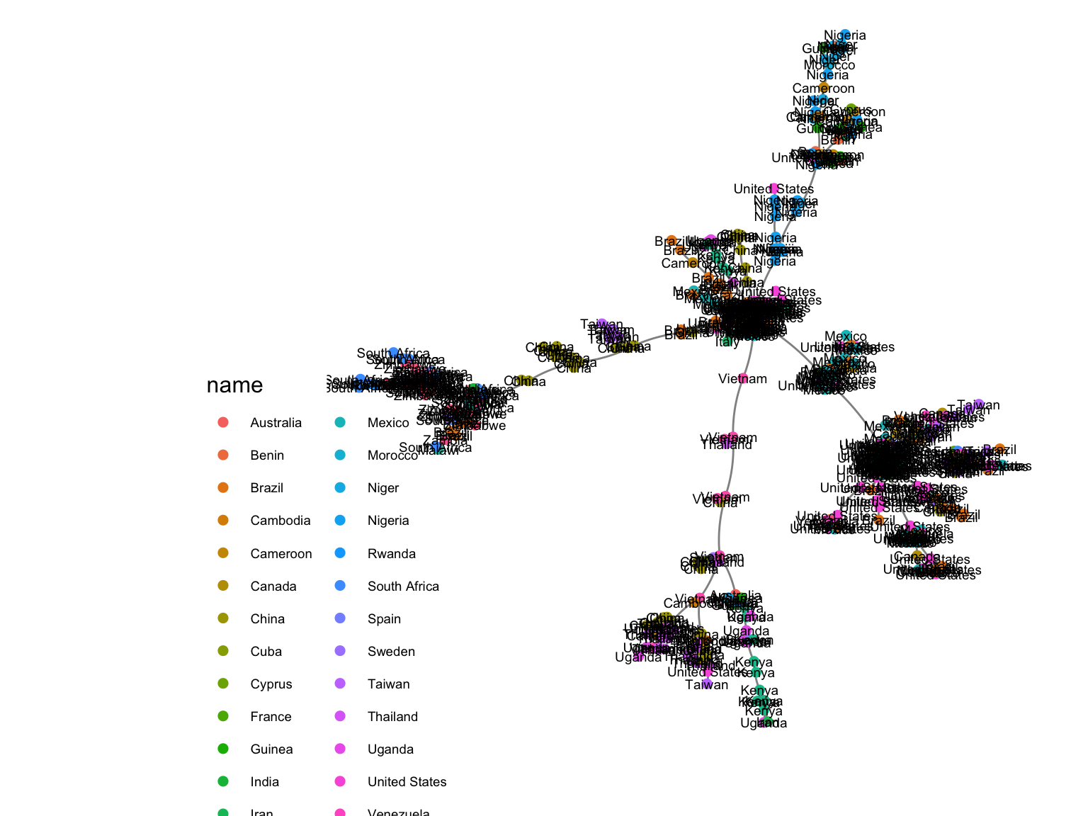

We can use the ggrepel package to make it cleaner:

ggplot(gg, aes(x = x, y = y, xend = xend, yend = yend)) +
  geom_edges(color = "black", alpha = 0.5, curvature = 0.1) +
  geom_nodes(aes(color = name), size = 2) +
  geom_nodetext_repel(aes(label = name), color="black", size = 2) +
  theme_blank() +
  guides(color = guide_legend(keyheight = 0.3, keywidth = 0.3,
         override.aes = list(size = 6), title = "Countries"))

A different approach to the layout for the MST: tidygraph and ggraph

More recently, there has been a new development with an extension of the ggraph package to include tidyverse compatible data structures, through the tidygraph package which creates “graph” tibbles.

library(tidygraph)
library(ggraph)
# Make sure you have the data loaded
# load(url("https://web.stanford.edu/class/bios221/data/dist2009c.RData"))
country09 <- attr(dist2009c, "Label")
class(dist2009c)

## [1] "dist"

graph09 <- graph_from_adjacency_matrix(as.matrix(dist2009c), weighted=TRUE)
mstree2009tidy <- igraph::mst(graph09)%>%as_tbl_graph()
## Without the labels

ggt<-ggraph(mstree2009tidy, layout = 'nicely') + geom_edge_link() + 
  theme_graph()
ggt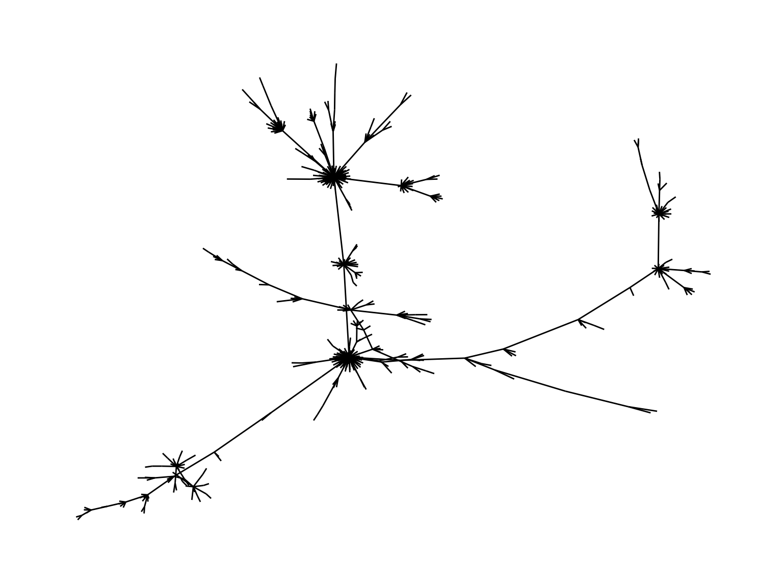

## Adding labels
ggt+
geom_node_text(aes(label = name), colour = 'purple', vjust = 0.4)+     theme_graph()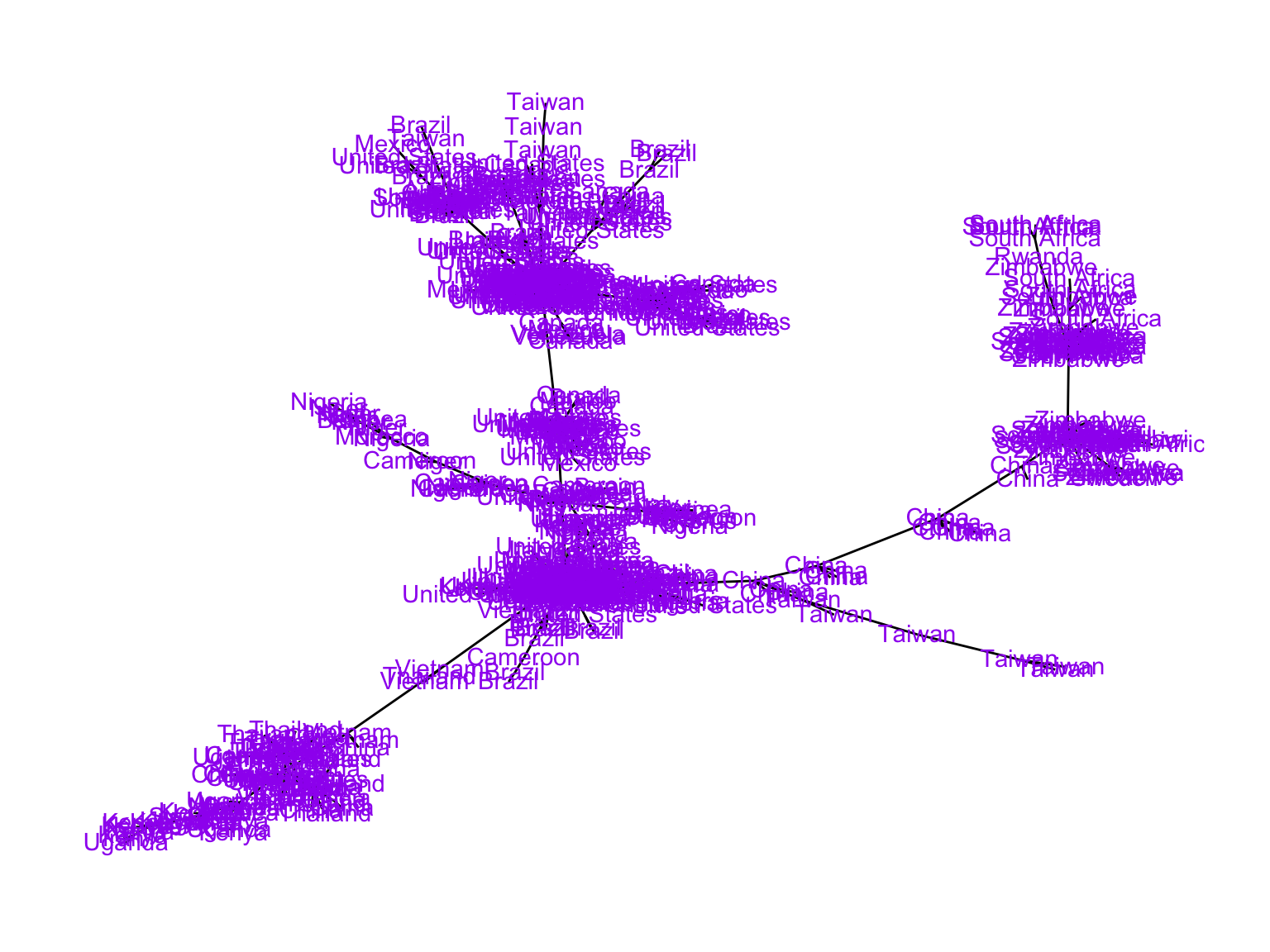

## Adding colors for countries
ggt+
geom_node_point(aes(color = name), size = 2) +theme_graph()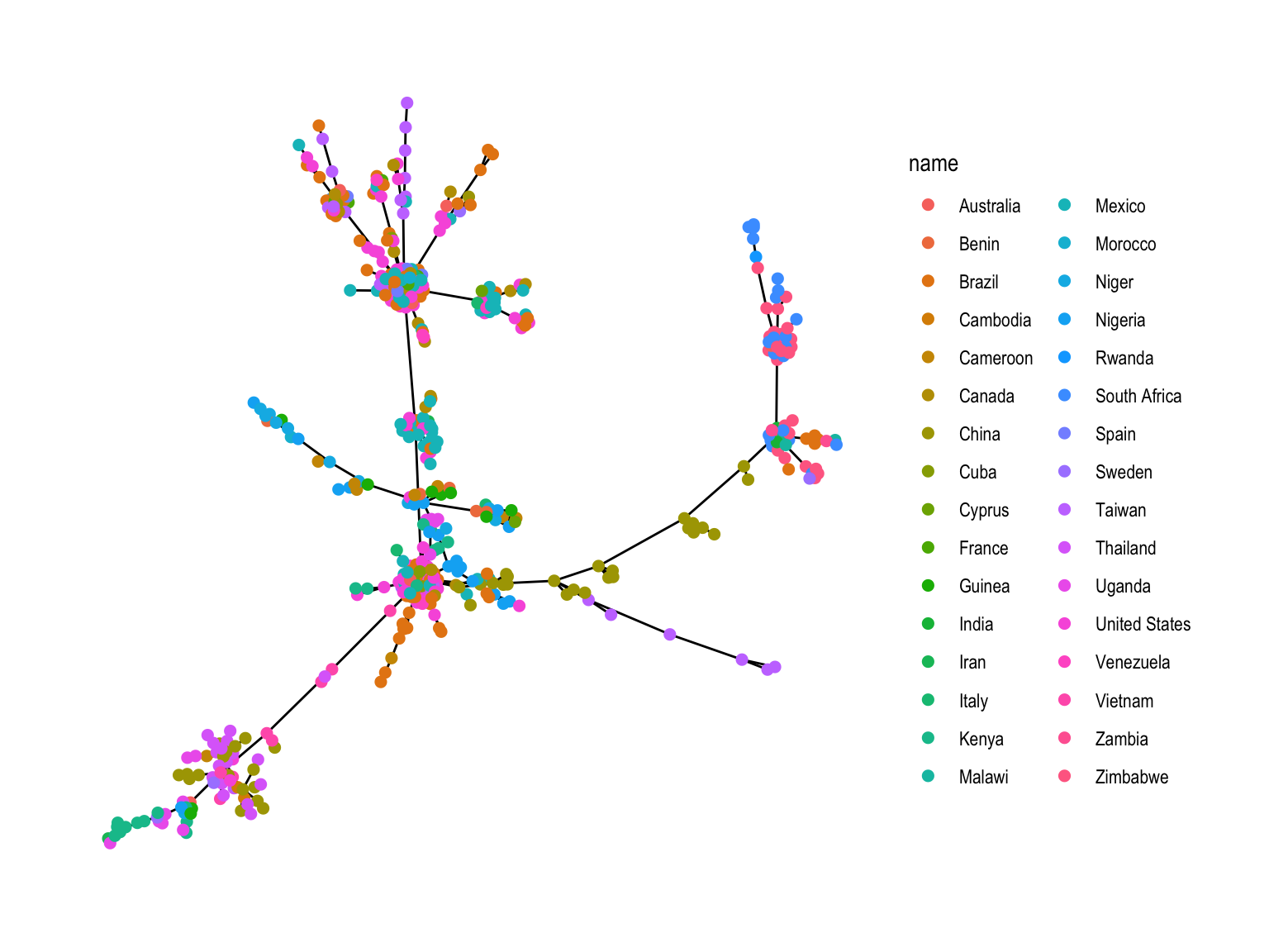

We would like to label only the countries which appear as hubs (ie with a high degree, say larger than 5).

We are going to compute the degrees and label the nodes according to their degrees. Let’s look at how to add that variable:

mstDegreed<-mstree2009tidy %>%
  activate(nodes) %>%
  mutate(degree=centrality_degree(,mode="all"))
mstDegreed

## # A tbl_graph: 512 nodes and 511 edges
## #
## # A rooted tree
## #
## # Node Data: 512 x 2 (active)
##   name     degree
##   <chr>     <dbl>
## 1 Thailand      1
## 2 Mexico        1
## 3 Zimbabwe      1
## 4 Taiwan        1
## 5 India         1
## 6 Mexico        1
## # … with 506 more rows
## #
## # Edge Data: 511 x 3
##    from    to weight
##   <int> <int>  <dbl>
## 1     7   145 0.0375
## 2     7   213 0.0269
## 3     7   228 0.0402
## # … with 508 more rows

Exercise

Try to modify the plotting code so that the labels of the higher degree hubs are larger and the graph nodes are readable:

ggraph(mstDegreed,layout = 'nicely') + geom_edge_link() + 
geom_node_point(aes(color = name))+ 
geom_node_text(aes(label = name, size=degree))+
theme_graph()

ggraph(mstDegreed,layout = 'nicely') + geom_edge_link() + 
geom_node_point(aes(color = name))+ 
geom_node_text(aes(label = name, size=degree,alpha=degree),nudge_x=-13,nudge_y=-6.5)+
theme_graph()

Remapping the minimum spanning tree on the world

We are going to make a minimum spanning tree between HIV cases using the geographic location of each case was made to reduce overlapping of points; the DNA distances between patient strains were used as the input to an undirected minimum spanning tree algorithm, the world coordinates come from the rworldmap package.

library("rworldmap")

mat <- match(country09, countriesLow$NAME)
coords2009 = data.frame(
  lat = countriesLow$LAT[mat],
  lon = countriesLow$LON[mat],
  country = country09)

layoutCoordinates = cbind(
  x = coords2009$lon,
  y = coords2009$lat)

ggt<-ggraph(mstree2009tidy, layout =   layoutCoordinates) +
  geom_edge_link() +
  theme_graph()
ggt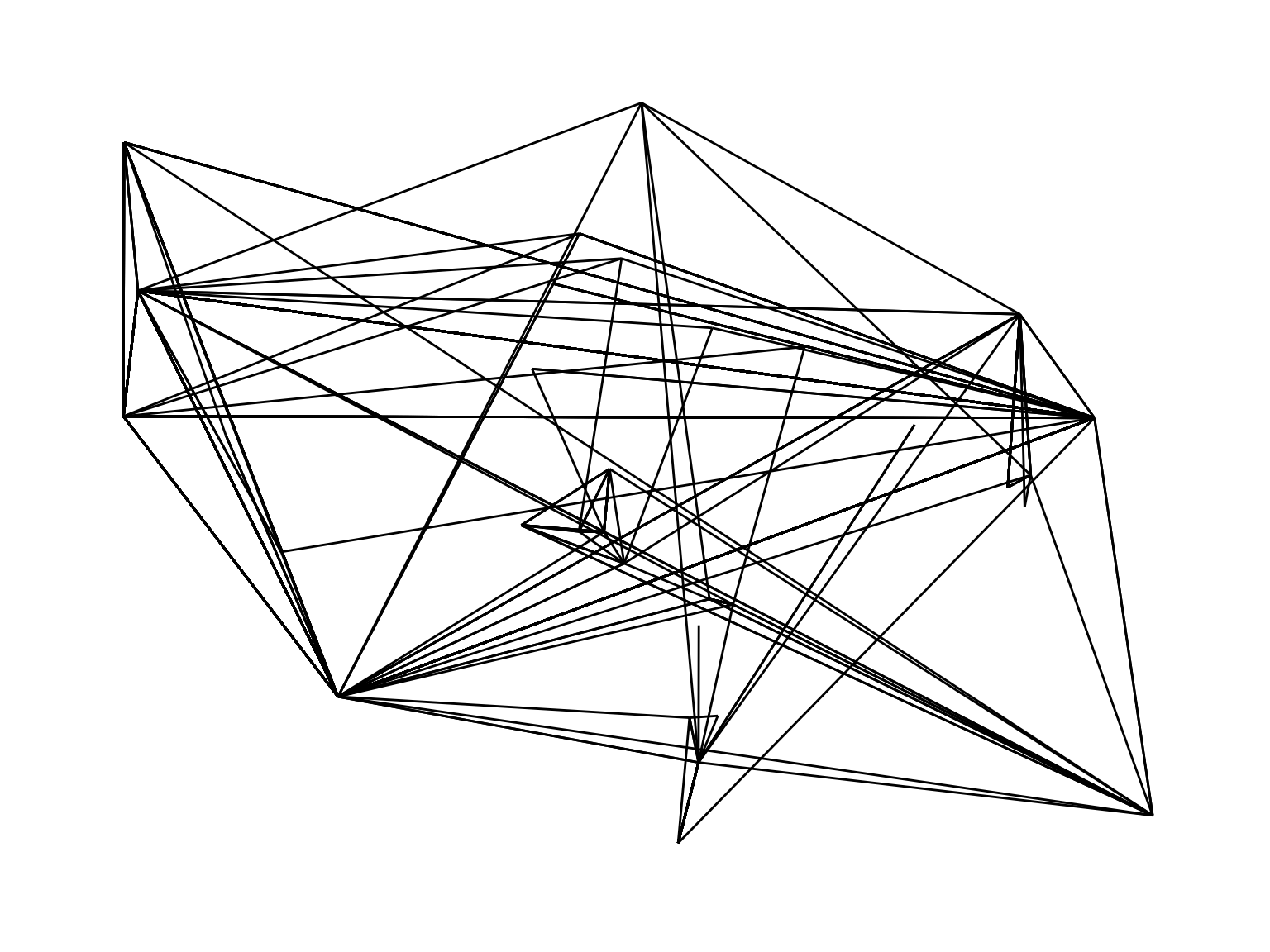

ggt<-ggraph(mstree2009tidy, layout = layoutCoordinates) + 
  geom_edge_link(alpha=0.3) + 
     theme_graph()
ggt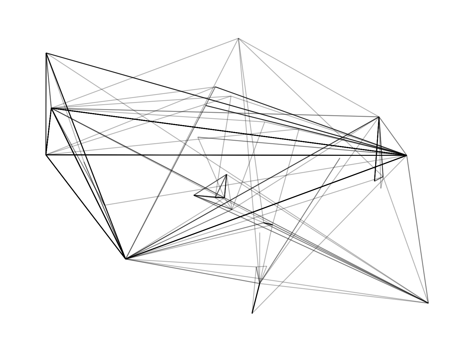

When comparing these two graphs, what do we notice?

Alot of overlapping edges that are invisible.

How can we fix this?

One way is to use jitter for each of the points.

Try modifying the code to add a jitter and plot a more instructive version of the graph.

jitterlayoutCoordinates = cbind(
  x = jitter(coords2009$lon, amount = 10),
  y = jitter(coords2009$lat, amount = 7))

ggt<-ggraph(mstree2009tidy, layout =   jitterlayoutCoordinates) +
  geom_edge_link(alpha=0.5,linemitre=5) +
  theme_graph()

We actually need to keep the jittered coordinates and assign the labels to the nodes so they appear on the plot.

labc = names(table(country09)[which(table(country09) > 1)])
matc = match(labc, countriesLow$NAME)
dfc = data.frame(
  latc = countriesLow$LAT[matc],
  lonc = countriesLow$LON[matc],
  labc)

ggt <- ggraph(mstree2009tidy, layout =   jitterlayoutCoordinates) +
geom_edge_link(alpha=0.5,linemitre=5) +
geom_label(data = dfc, aes(x = lonc, y = latc, label = labc, fill = labc), colour = "white", alpha = 0.7, size = 3) +
  geom_node_point(aes(color = country09), size = 2,alpha=0.4) + guides(fill=FALSE)+
    theme_graph()
ggt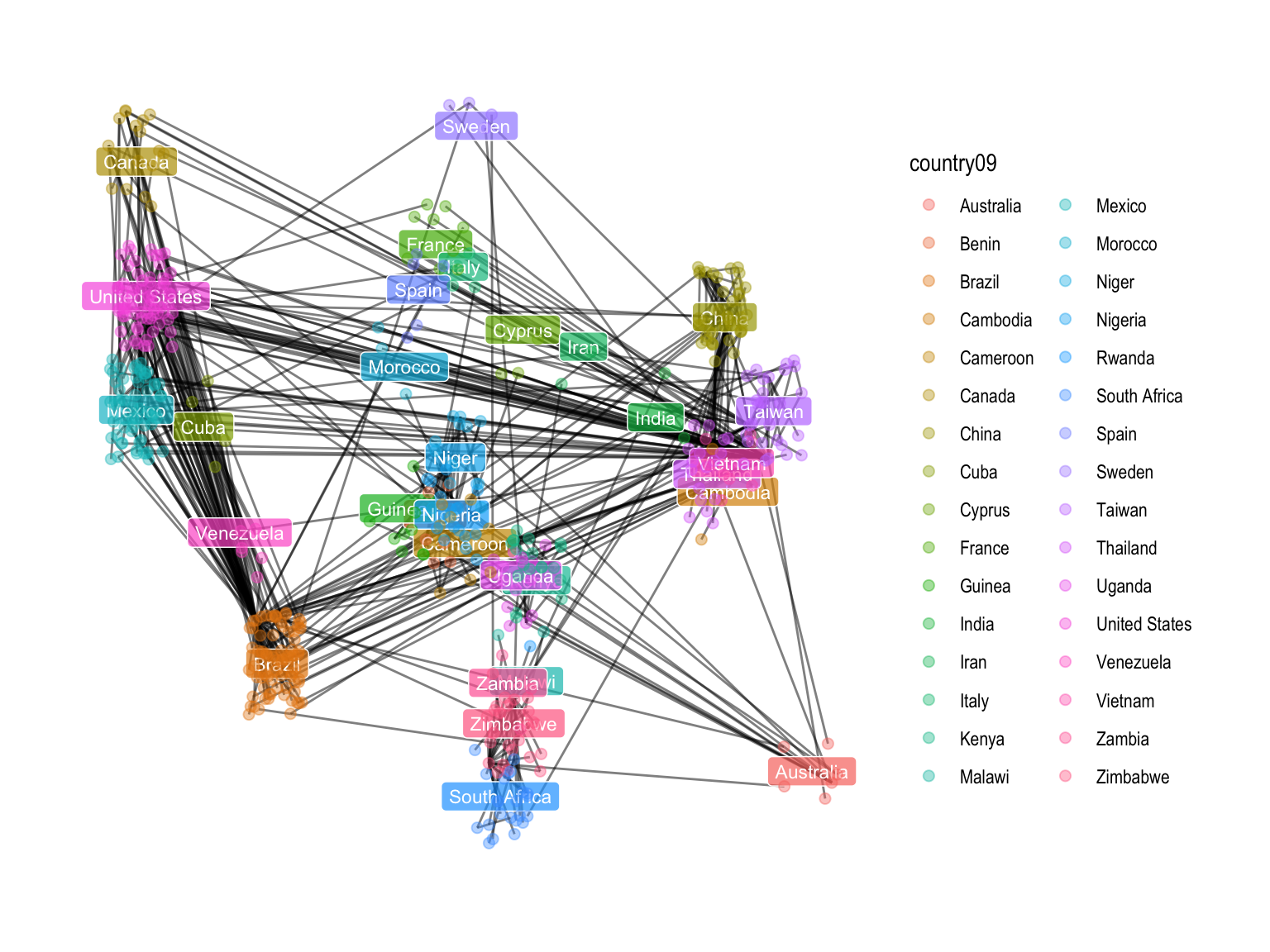

Try changing the type of edge (bend,diagonal,arc)

ggt <- ggraph(mstree2009tidy, layout =   jitterlayoutCoordinates) +
geom_edge_link(alpha=0.5,linemitre=5) +
geom_label(data = dfc, aes(x = lonc, y = latc,label = labc, fill = labc), colour = "white", alpha = 0.7, size = 3) +
  geom_node_point(aes(color = country09), size = 2,alpha=0.4) +
  guides(fill=FALSE)+
    theme_graph()
ggt

ggt <- ggraph(mstree2009tidy, layout =   jitterlayoutCoordinates) +
geom_edge_bend(alpha=0.5,linemitre=5) +
geom_label(data = dfc, aes(x = lonc, y = latc,label = labc, fill = labc), colour = "white", alpha = 0.7, size = 3) +
  geom_node_point(aes(color = country09), size = 2,alpha=0.4) +
  guides(fill = FALSE) +
    theme_graph()
ggt

Another new possibility is the new sfnetworks package which allows for paths and routing

Co-occurrence graphs

We are going to look at microbial abundances of different strains/species of bacteria in biological samples.

These samples come from a longitudinal study of mice from several litters.

Bacterial community example using a phyloseq object

We load the phyloseq package first and read the phyloseq object that integrates all the data.

library("phyloseq")
#External file
ps1  = readRDS(url("https://web.stanford.edu/class/bios221/data/ps1.rds"))
#Internal file from package data
# data(ps1)
ps1

## phyloseq-class experiment-level object
## otu_table()   OTU Table:         [ 389 taxa and 344 samples ]
## sample_data() Sample Data:       [ 344 samples by 16 sample variables ]
## tax_table()   Taxonomy Table:    [ 389 taxa by 6 taxonomic ranks ]
## phy_tree()    Phylogenetic Tree: [ 389 tips and 387 internal nodes ]

We could like to connect the samples that have a lot of bacteria in common. The best way to measure similarity between species abundances is the “Jaccard distance”.

We start by computing the Jaccard distance between samples and set a threshold for the distance to correspond to an edge in the “co-occurrence” graph.

Exercise: Add a line of code that makes the shape give the litter information:

# data(ps1)
ps1
ig<-make_network(ps1, max.dist=0.3)
plot_network(ig,ps1,color="host_subject_id")

We can replicate what the function is doing by hand, using the tidygraph package, you have to add a few lines to remove the isolates.

We start by checking the libraries

require("tidygraph")
require("igraph")
require("ggraph")

Then we make an igraph object and make the graph into a tidygraph (tbl):

d1 <- as.matrix(phyloseq::distance(ps1, method="jaccard"))
d1 <- d1 +diag(ncol(d1))
threshM <- (d1<0.35)
gr <- graph_from_adjacency_matrix(threshM,  mode = "lower")
sampledata = data.frame( sample_data(ps1))
V(gr)$id = sampledata[names(V(gr)), "host_subject_id"]
V(gr)$litter = sampledata[names(V(gr)), "family_relationship"]
tigr<- gr%>% as_tbl_graph()
tigr
ggraph(tigr,layout="fr")+ geom_edge_link() +
  geom_node_point(aes(color=id,shape=litter))+
  theme_graph()

Testing a graph for association with a factor variable

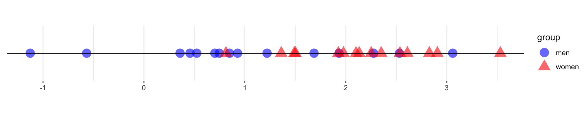
For univariate data in two groups, we can test the differences by looking at the number of runs within each group.

Seeing the number of runs in a one-dimensional, two-sample, nonparametric Wald-Wolfowitz test can indicate whether the two groups have the same distributions.

Testing the relation between a graph and vertex factors

The samples have factor covariates

The nodes in the graph correspond to the samples and are associated to factors that specify the litter and individual ids of the mice from which the samples were collected.

library("phyloseq")
library("phyloseqGraphTest")
library("igraph")
## data(ps1)
ps1  = readRDS(url("https://web.stanford.edu/class/bios221/data/ps1.rds"))
ps1

## phyloseq-class experiment-level object
## otu_table()   OTU Table:         [ 389 taxa and 344 samples ]
## sample_data() Sample Data:       [ 344 samples by 16 sample variables ]
## tax_table()   Taxonomy Table:    [ 389 taxa by 6 taxonomic ranks ]
## phy_tree()    Phylogenetic Tree: [ 389 tips and 387 internal nodes ]

sampledata = data.frame( sample_data(ps1))
d1 = as.matrix(phyloseq::distance(ps1, method="jaccard"))
gr = graph.adjacency(d1,  mode = "undirected", weighted = TRUE)
net = igraph::mst(gr)
V(net)$id = sampledata[names(V(net)), "host_subject_id"]
V(net)$litter = sampledata[names(V(net)), "family_relationship"]

The minimum spanning tree based on Jaccard dissimilarity and annotated with the mice ID and litter factors.

library(ggnetwork)
gnet=ggnetwork(net)
ggplot(gnet, aes(x = x, y = y, xend = xend, yend = yend))+
  geom_edges(color = "darkgray") +
  geom_nodes(aes(color = id, shape = litter)) + theme_blank()+
  theme(legend.position="bottom")

library("phyloseqGraphTest")
gt = graph_perm_test(ps1, "host_subject_id", distance="jaccard",
                     type="mst",  nperm=1000)
plot_test_network(gt)

gt

## Output from graph_perm_test
## ---------------------------
## Observed test statistic: 149 pure edges
## 343 total edges in the graph
## Permutation p-value: 0.000999000999000999

plot_permutations(gt)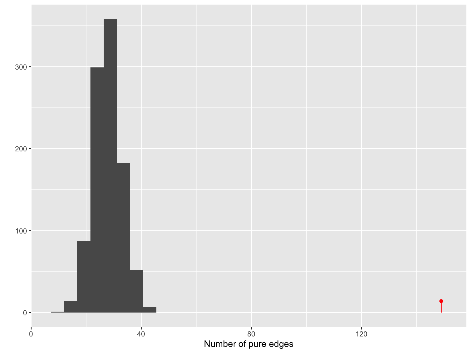

gt$pval

## [1] 0.000999001

The permutation histogram of the number of pure edges in the network obtained from the minimal spanning tree with Jaccard similarity.

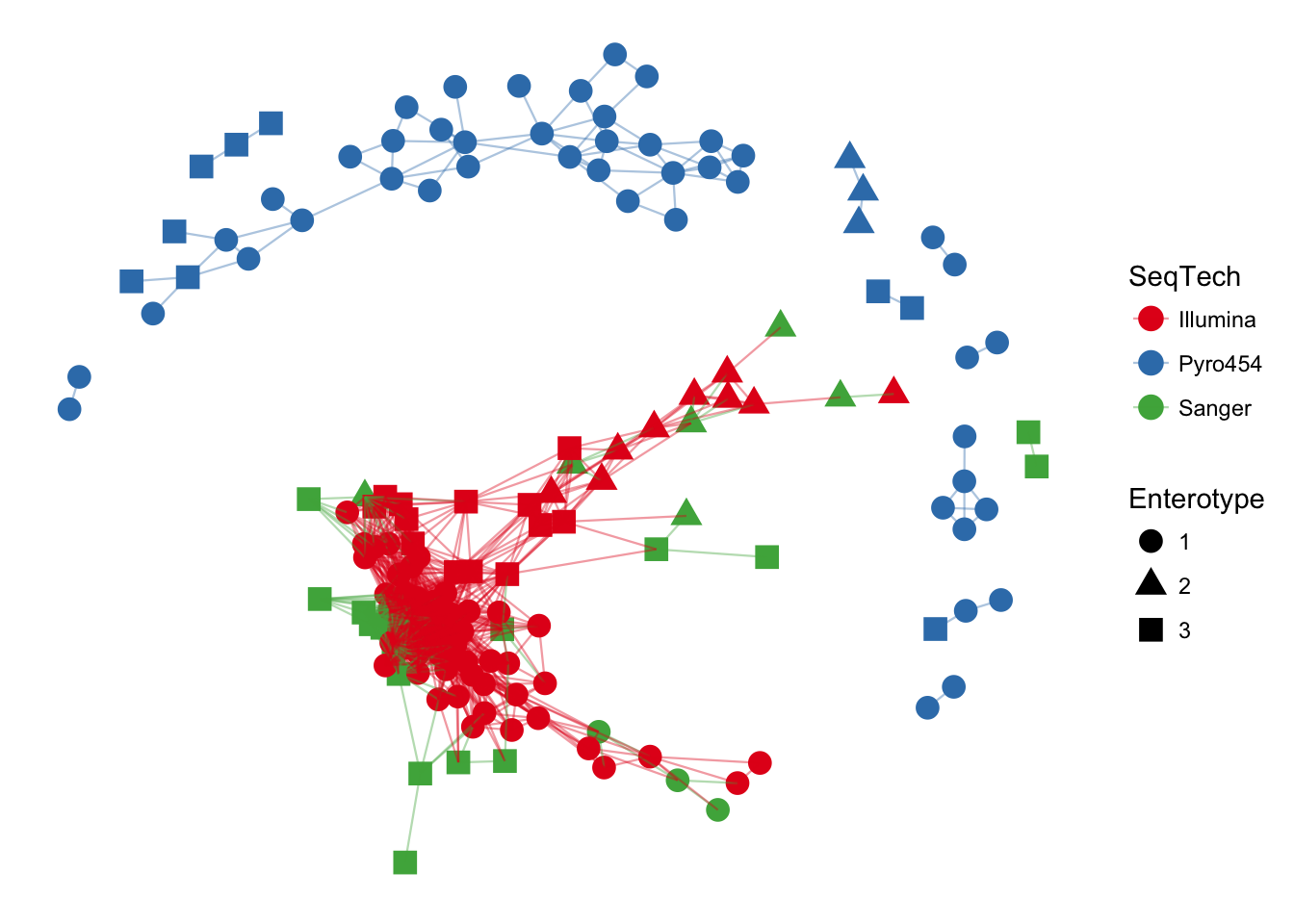
net = make_network(ps1, max.dist = 0.35)
sampledata = data.frame(sample_data(ps1))
V(net)$id = sampledata[names(V(net)), "host_subject_id"]
V(net)$litter = sampledata[names(V(net)), "family_relationship"]
netg = ggnetwork(net)

ggplot(netg, aes(x = x, y = y, xend = xend, yend = yend)) +
  geom_edges(color = "darkgray") +
  geom_nodes(aes(color = id, shape = litter)) + theme_blank()+
    theme(plot.margin = unit(c(0, 5, 2, 0), "cm"))+
    theme(legend.position = c(1.4, 0.3),legend.background = element_blank(),
          legend.margin=margin(0, 3, 0, 0, "cm"))+
         guides(color=guide_legend(ncol=2))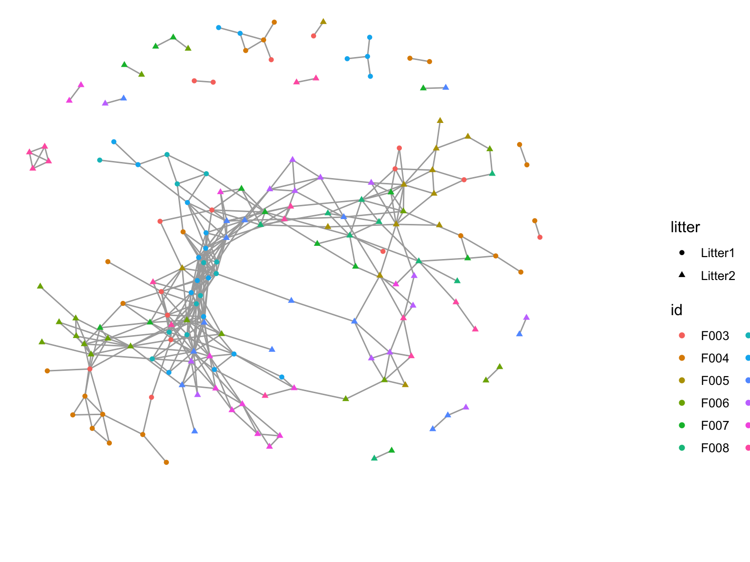

A co-occurrence network created by using a threshold on the Jaccard dissimilarity matrix. The colors represent which mouse the sample came from; the shape represents which litter the mouse was in.

gt = graph_perm_test(ps1, "family_relationship",
        grouping = "host_subject_id",
        distance = "jaccard", type = "mst", nperm= 1000)
gt$pval

## [1] 0.000999001

plot_permutations(gt)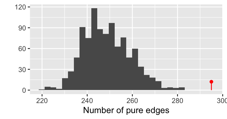

The permutation histogram obtained from the minimal spanning tree with Jaccard similarity.

gtnn1 = graph_perm_test(ps1, "family_relationship",
                      grouping = "host_subject_id",
                      distance = "jaccard", type = "knn", knn = 1)
gtnn1$pval

## [1] 0.004

plot_test_network(gtnn1)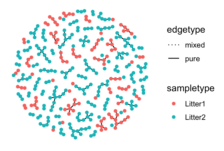

The graph obtained from a nearest-neighbor graph with Jaccard similarity.

References :

• Online book chapter of book by Holmes and Huber

• Tutorial on networks with phyloseq

phyloseq network

• tidygraph tutorial

tidygraph_hex.png

• phyloseqGraphTest vignette

• Friedman Rafsky explanation and details