The test case is run at the command line with the command
make testwhich runs the simulation for 3000 time steps (
suntans.dat: nsteps = 3000)
with a time step size of 29.808 s (suntans.dat: dt = 29.808) for a total of
2 sponge_distance = 5000 and
sponge_decay = 7200 (for details see Section 7).
The results can be viewed with the sunplot gui from the main source directory with
./sunplot --datadir=examples/iwaves/dataThis brings up a planview of the one-dimensional grid of equilateral triangles. To display the profile plot of the results, press the
 button with the middle mouse
button and then the
button with the middle mouse
button and then the
 button with the left mouse button so that the axes fill the plot window.
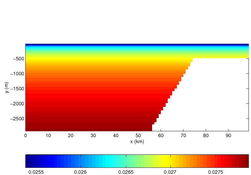
This will display the salinity (density) field at the first time step, as shown in Figure
15. Plotting the u-velocity at data steps 11 and 21 will display the horizontal
velocity field after one and two periods of forcing, respectively, as shown in Figures
16 and 17. Note that even with the use of the sponge layer,
some internal wave energy is reflected back from the left boundary and affects the internal
wave field shown in Figure 17. In addition to using
button with the left mouse button so that the axes fill the plot window.
This will display the salinity (density) field at the first time step, as shown in Figure
15. Plotting the u-velocity at data steps 11 and 21 will display the horizontal
velocity field after one and two periods of forcing, respectively, as shown in Figures
16 and 17. Note that even with the use of the sponge layer,
some internal wave energy is reflected back from the left boundary and affects the internal
wave field shown in Figure 17. In addition to using sunplot, printouts for
these plots can be obtained with the
plotslice.m m-file which can be downloaded from
http://suntans.stanford.edu/downloads_stanford .
|
0.75 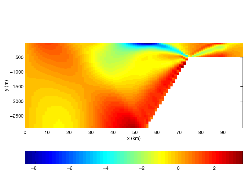
|
|
0.75 
|