Rethinking the Primitives: Next Generation LLM Architecture

The Architecture Stack

A language model is a stack. Tokens enter as embeddings, pass through some representation of their position, flow through dozens of alternating attention and feed-forward sublayers, are optionally routed through sparse expert banks, and emerge after a normalization step before the next layer begins. The same pattern repeats from the first layer to the last.

Almost every component in this stack has been accepted largely as-is since the original Transformer (Vaswani et al., 2017) — not because it is provably optimal, but because it works, and because revisiting it is costly. Rotary positional embeddings replaced absolute positions, but the attention operator underneath remained unchanged. Mixture-of-Experts replaced dense FFNs, but the Softmax router remained unchanged. Pre-Norm replaced Post-Norm for stability, but the structural question of what normalization is for was never addressed.

The works described here take a different approach: for each component, first ask what it is mathematically doing, then ask whether the conventional implementation is the best realization of that function. In each case, the answer is no — and the better design follows almost directly from the mathematical analysis.

Traversing the stack from input representation to training stability:

• Positional encoding: Standard PE schemes inject position into query/key vectors before the dot product. DAPE V2 asks what should happen to positional information after the dot product — and finds that the attention score tensor, viewed as a feature map, benefits from convolution across heads.
• Attention mechanisms: Performance scales with the number of attention heads, but so do parameter counts. SAS decouples the two by projecting into higher-dimensional spaces to simulate more heads than the model actually has.
• Linear hybrid attention: O(n²) attention is prohibitively expensive for long generation. The Gated Memory Unit (GMU) enables cross-layer hidden-state sharing in a purely SSM model, yielding the SambaY architecture that achieves reasoning-Transformer performance with linear decoding complexity.
• Mixture-of-Experts routing: The Softmax router, standard since Switch Transformer, is mathematically equivalent to Nadaraya-Watson kernel regression with the exponent kernel. KERN shows this kernel is suboptimal and proposes a better one at zero cost.
• Normalization: Pre-Norm and Post-Norm each sacrifice something — stability or expressiveness. GeoNorm reveals both as first-order approximations of a geodesic update on the unit sphere manifold, and computes the exact geodesic instead.

This is a vertical slice through the entire Transformer stack. The connecting thread is not a single technique but a methodology: find the hidden mathematical structure, then design from it.

Positional Encoding: DAPE V2

The Length Extrapolation Problem

Train a Transformer on sequences of length 2048. Ask it to process length 8192. In most cases, performance degrades — sometimes catastrophically. This is the length extrapolation problem, and it has spawned an industry of positional encoding variants: ALiBi adds a linear distance bias; RoPE rotates query and key vectors by position-dependent angles; YaRN and LongRoPE extend RoPE's range through rescaling.

But these solutions all operate at the same level of abstraction — they modify what gets added to or multiplied by the query and key vectors before the dot product. DAPE V2 asks a different question: what if the bottleneck is not what gets added, but the operator itself?

The Expressiveness Bottleneck

Standard attention computes, for each head $h$:

This single scalar $A^h_{ij}$ is expected to encode both the semantic relationship between positions $i$ and $j$, and their positional relationship. A dot product is a symmetric, bilinear form — a relatively weak operator. For tokens whose distance exceeds the training range, the positional component of $q_i^h \cdot k_j^h$ falls in an extrapolation regime the model has never optimized over, which is exactly why performance degrades.

CDAPE: Convolution Across Heads

CDAPE (Convolutional DAPE) treats the $H$-channel attention score tensor as a feature map and applies a 1D convolution along the head axis:

Here $w$ is a learnable filter of kernel size $k$ (in practice $k=3$ or $5$), shared across all positions $(i,j)$. The convolution mixes nearby heads' attention scores — head $h$ can borrow information from heads $h\pm 1, h\pm 2$. Because $w$ is position-agnostic, the same filter applies regardless of the absolute indices $i$ and $j$, which is exactly what enables generalization to longer sequences.

# CDAPE: apply 1D conv across the head dimension of attention scores
# scores: [B, H, N, N] — standard pre-softmax attention logits

B, H, N, _ = scores.shape
# reshape so head axis is the "channel" for 1D conv
x = scores.permute(0, 2, 3, 1).reshape(B * N * N, 1, H)
x = self.conv1d(x)                      # depthwise conv, kernel k
delta = x.reshape(B, N, N, H).permute(0, 3, 1, 2)

scores = scores + delta                 # additive residual
attn   = F.softmax(scores, dim=-1)
output = attn @ V

Why do different attention heads correlate in the ways that make cross-head convolution useful? Attention heads are known to specialize — syntactic heads, positional heads, semantic heads. These specializations are not independent: a head that learns to attend to immediate neighbors likely produces attention scores that covary with heads attending to slightly more distant neighbors. The convolution exploits this inter-head correlation structure, effectively allowing each head to have a richer, context-aware view of positional relationships.

The result is consistent improvement in length extrapolation across benchmarks — and, interestingly, improved performance even at training-range lengths, since the cross-head interaction adds expressiveness beyond position.

Attention Mechanism: SAS

The Head Count Dilemma

Attention performance scales with both the number of heads $H$ and the per-head dimension $d_k$. More heads means more diverse attention patterns; larger $d_k$ means each head can represent richer query-key relationships. The problem: in standard multi-head attention, $d_k = d_\text{model}/H$, so the two are in direct tension at fixed model size. Doubling $H$ halves $d_k$.

The implicit assumption is that expressiveness must come from parameters. SAS questions this assumption: can we decouple the number of effective attention patterns from the number of parameter heads?

Simulation Through Projection

SAS generates $s$ virtual attention maps from each real head by projecting queries and keys into diverse higher-dimensional spaces:

where $W_{\text{sim}} \in \mathbb{R}^{d_k \times \tilde{d}_k}$ is a learned projection. Each pair $(W_{\text{sim},Q}^{h,i}, W_{\text{sim},K}^{h,i})$ rotates and (optionally) expands the head's representation, yielding an attention map that explores a different "view" of the same token features. With simulation factor $s$, the model effectively has $s \cdot H$ attention patterns while paying the parameter cost of only $H$ heads plus $2sH$ small projection matrices.

The intuition is close to random Fourier features in kernel methods: by projecting into a higher-dimensional space, you can approximate the behavior of a larger model without paying the full parameter cost. The projections are learned, not random, so they adapt to the data distribution.

PEAA: Aggregating Without Overhead

With $s \cdot H$ simulated attention maps, they must be recombined. SAS uses Parameter-Efficient Attention Aggregation (PEAA): a learned static mixture over the $s$ simulated heads per real head,

where $\mathbf{g}^h \in \mathbb{R}^s$ are scalar gate parameters (one per simulated head). The gate is input-independent — it is a fixed mixture weight, not a function of the token — which keeps PEAA free of additional attention computation. The overhead over standard MHA is just $s$ scalars per real head: negligible.

DAPE V2 and SAS are complementary. DAPE V2 enriches attention by applying a learned operator after the dot product (in score space, across heads). SAS enriches attention by applying learned projections before the dot product (in feature space, within each head). Both decoupled expressiveness from raw parameter count; both can be applied simultaneously.

Linear Hybrid Attention: Decoder-Hybrid-Decoder and SambaY

Two Models, Two Tradeoffs

Transformers and State Space Models (SSMs, e.g., Mamba) represent opposite ends of a tradeoff. Transformers store the entire context in a KV-cache that grows linearly with generation length. This gives exact recall of any past token — powerful for retrieval and precise reasoning — but memory and compute scale as $O(n)$ per step, making long generation expensive. SSMs maintain a fixed-size hidden state regardless of context length, enabling constant-memory autoregressive decoding and $O(n)$ pre-filling — but their finite-capacity state means information from many steps back may be lossy or forgotten.

For extended chain-of-thought reasoning — where models generate thousands of tokens — this tradeoff is acute. You want efficient decoding (SSM), but you also want to reliably recall an intermediate result computed 500 tokens ago (Transformer). Hybrid architectures that interleave SSM and attention layers help, but the key question is: how should the SSM and attention components communicate?

The Gated Memory Unit

Prior hybrids treat SSM and attention layers as independent — information flows only through the residual stream (token representations). The Gated Memory Unit (GMU) adds a direct pathway between the hidden states of SSM layers at different depths:

where $h_t^{(\ell)}$ is the SSM hidden state at layer $\ell$ and $h_t^{(\ell')}$ is the state at a downstream layer $\ell' > \ell$. The sigmoid gate $\sigma(W_g h_t^{(\ell)})$ selects which components of the upstream state are relevant to pass forward. This is a form of residual memory: the hidden state, not just the token representation, can shortcut across layers.

Why does this matter for reasoning? A chain of thought establishes facts at different steps: "We know $x = 3$, therefore $2x = 6$, therefore $y = 2x + 1 = 7$." Each fact is encoded in the SSM hidden state when it is computed. Without GMU, that encoding must survive multiple layers of SSM compression before it is accessible. With GMU, the state encoding a critical intermediate result can be directly injected into later states — a form of selective working memory.

SambaY and Phi4-mini-Flash-Reasoning

SambaY Architecture

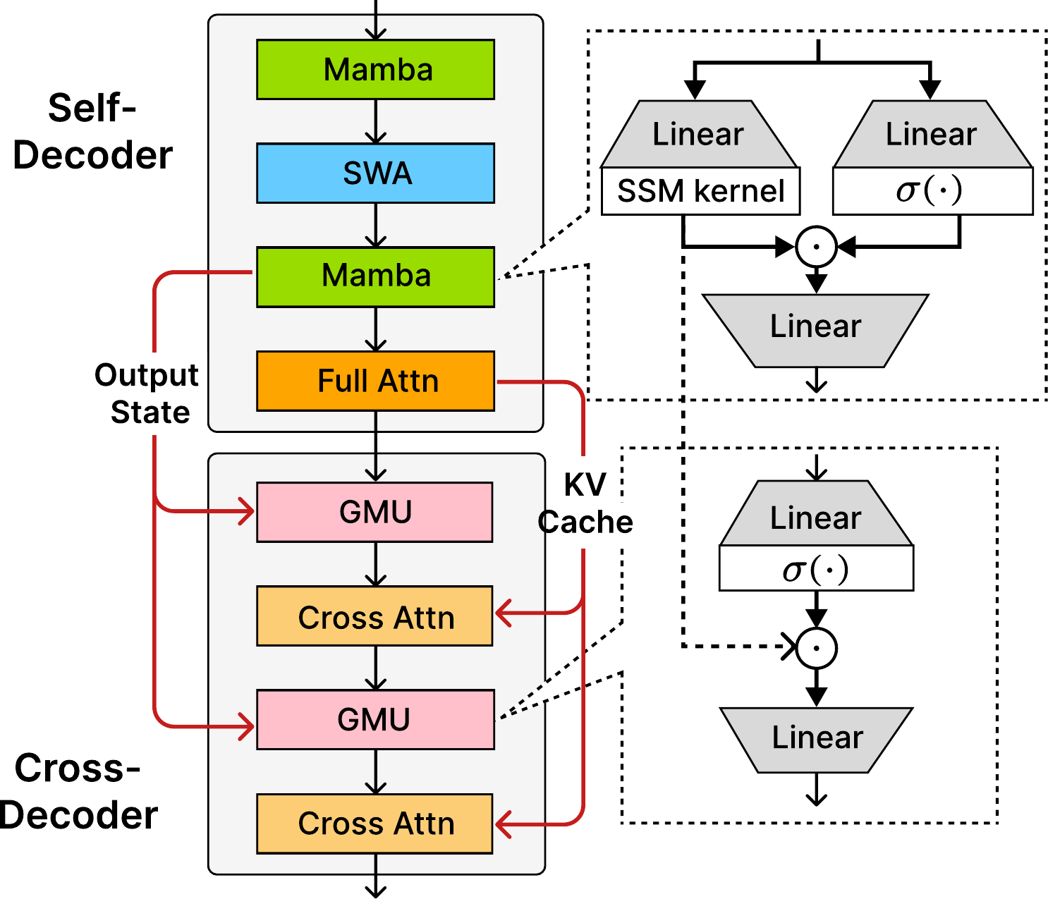
SambaY takes its name from its Y-shaped structure. The Self-Decoder is a hybrid stack of Mamba SSM and attention layers (Mamba → SWA → Mamba → Full Attention). It processes the input sequence and produces two outputs that branch into the Cross-Decoder: (1) an Output State — the SSM hidden state from the final Mamba layer — which is injected into each GMU block in the Cross-Decoder, and (2) a KV Cache from the Full Attention layer, which feeds each Cross-Attention block. The Cross-Decoder alternates GMU and Cross-Attention layers, using both channels to condition its generation on the Self-Decoder's compressed representations. This dual-channel conditioning is the "Y": one branch carries recurrent state memory, the other carries token-level attention context.

Phi4-mini-Flash-Reasoning uses SambaY as its backbone. Compared to Phi4-mini-Reasoning (a Transformer-based model trained with RL on verifiable rewards), Phi4-mini-Flash-Reasoning achieves significantly better results on Math500, AIME 2024/25, and GPQA Diamond — with up to 10× higher decoding throughput in long generation scenarios. These gains come entirely from architecture, not from reinforcement learning post-training.

Mixture-of-Experts Routing: KERN

MoE and the Unquestioned Softmax

Mixture-of-Experts models route each token to a subset of specialized FFN experts via a router. Since the original Switch Transformer, the router has invariably been a linear layer followed by Softmax:

Softmax has never been seriously questioned as the router design. It is borrowed from classification — which is not obviously the right inductive bias for token routing. This paper asks: what is the right design, and why?

The Nadaraya-Watson Connection

Nadaraya-Watson (NW) regression is a classical nonparametric estimator. Given data $\{(x_i, y_i)\}$, it estimates the conditional mean as a kernel-weighted average of outputs:

The connection to MoE is exact: identify each expert $E_k$ with a training output $y_k$, and each router weight vector $w_k$ with a training input $x_k$. Then $G_k(x) = K(x, w_k) / \sum_{k'} K(x, w_{k'})$, and MoE(x) = NW regression on the experts. Both standard FFNs (with ReLU nonlinearity) and MoE are special cases of NW regression with different kernels. Softmax-routed MoE corresponds to the exponent kernel $K(x, w) = e^{w^\top x}$.

The KERN Router

The exponent kernel $K(x,w) = e^{w^\top x}$ has a problematic property: it is always positive. Every expert receives nonzero weight for every token — there is no principled mechanism for a token to "abstain" from routing to irrelevant experts. This leads to the need for explicit load-balancing auxiliary losses.

KERN proposes a better kernel: ReLU activation with ℓ₂-normalized router weights.

$\hat{w}_k^\top x$ is the cosine similarity between the (normalized) router prototype and the token. ReLU sets this to zero when the token is on the "wrong side" of the expert's hyperplane — the expert is simply inactive, with no gradient pulling it to take a nonzero weight. The normalization ensures that active expert weights sum to 1, as in Softmax. KERN thus inherits sparsity from ReLU and normalization from Softmax, while being a strict generalization of both.

# KERN router: cosine similarity + ReLU + normalize
W_hat = F.normalize(self.W, dim=-1)         # [K, d] — L2-norm rows
logits = x @ W_hat.t()                      # [B, N, K] cosine sims
gates  = F.relu(logits)                     # exact zeros for inactive experts
gates  = gates / gates.sum(-1, keepdim=True).clamp(1e-8)

KERN achieves consistent perplexity improvements over Softmax routing across model scales and tasks, with zero additional FLOPs. The ℓ₂ normalization of $W$ can be precomputed and cached, so inference cost is identical to Softmax routing.

Normalization: GeoNorm

The Normalization Placement Debate

Two normalization placements have competed since Transformers were introduced. Post-Norm (original Transformer) applies LayerNorm after the residual addition:

Pre-Norm applies LayerNorm to the sublayer input:

Post-Norm is more expressive — the raw sublayer output $F(x_t)$ is allowed to be large, so each layer can make substantial transformations. But Post-Norm is hard to train: deep Post-Norm networks often diverge without careful warmup and initialization. Pre-Norm is stable but leaves a persistent performance gap. Every major LLM (GPT-3, LLaMA, Mistral) uses Pre-Norm not because it is optimal but because it is trainable.

The Geometric Perspective

The key insight is to interpret representations as living on the unit sphere $\mathcal{S}^{d-1}$. LayerNorm (with zero mean, unit variance) projects token representations to approximately unit norm — near-spherical. The sublayer output $\delta = F(\mathrm{LN}(x_t))$ is an update direction on this sphere.

On the sphere, the natural update is a geodesic — the shortest arc-length path between two points. Moving from $x_t$ in direction $\delta$ along the geodesic for a step of size $\alpha\|\delta\|$ gives exactly:

This is the spherical interpolation (slerp) formula. It moves from $x_t$ toward $\delta$ along the sphere's surface, arriving at a unit-norm result by construction — no normalization needed post hoc.

Pre-Norm and Post-Norm as Approximations

Both normalization schemes are now revealed as approximations of this geodesic. Expanding the geodesic to first order in $\alpha$:

This is exactly Pre-Norm with step size $\alpha$. Pre-Norm is the first-order Taylor approximation of the geodesic — stable precisely because small $\alpha$ keeps $\|\alpha\delta\|$ small, so the approximation error is small.

Post-Norm, on the other hand, takes the Euclidean step $x_t + F(x_t)$ and projects back to the sphere via LN. This is a chord-to-arc projection: take a straight-line step and snap back to the surface. When the Euclidean step is large (expressive Post-Norm behavior), the projection introduces error relative to the true geodesic — but also allows the update to "reach further" than Pre-Norm's small step. Both are approximations; neither is the exact geodesic.

GeoNorm: Computing the Geodesic Directly

def geonorm(x, delta, alpha):
    """
    x:     residual stream, ~unit norm  [B, N, d]
    delta: sublayer output F(LN(x))    [B, N, d]
    alpha: learnable scalar step size (initialized small)
    """
    norm  = delta.norm(dim=-1, keepdim=True).clamp(1e-8)
    theta = alpha * norm               # angle to travel
    d_hat = delta / norm               # unit direction
    return torch.cos(theta) * x + torch.sin(theta) * d_hat

GeoNorm replaces the residual addition with this exact geodesic computation. The scalar $\alpha$ (one per sublayer) is a learnable step size, initialized small (Pre-Norm regime). As training proceeds, each layer learns the optimal step — early layers tend to learn small $\alpha$ (stable, Pre-Norm-like) while later layers can learn larger steps where the task requires more substantial transformation.

A layer-wise decay schedule $\alpha_\ell = \alpha_0 \cdot \gamma^\ell$ provides an inductive bias: deeper layers, being closer to the output, update more conservatively. This mirrors the well-known practice of using smaller learning rates for layers nearer the output in transfer learning.

GeoNorm is a strict generalization: Pre-Norm and Post-Norm are its limiting cases. In experiments, GeoNorm consistently outperforms both, closing the expressiveness gap of Pre-Norm without the instability of Post-Norm.

The Bigger Picture

The Transformer stack is not a fixed point. It is a collection of engineering decisions made under uncertainty, each encoding an implicit assumption about what operation is needed. Looking at those assumptions carefully, layer by layer:

• Positional encoding assumed that position is best injected into QK features before the dot product. DAPE V2 shows the dot product output — the attention score — is itself a rich feature map that benefits from further processing.
• Attention mechanisms assumed that expressiveness must come from parameter count. SAS shows that projection into higher-dimensional spaces decouples the two, giving more expressive attention at the same cost.
• Sequence modeling assumed a binary choice between O(n²) attention (expressive, slow) and O(1)-state SSMs (fast, forgetful). Decoder-Hybrid shows the dichotomy is false: a GMU-connected SSM stack achieves Transformer-level reasoning at linear decoding cost.
• MoE routing assumed that Softmax is the natural operator for token-to-expert assignment. KERN shows it is just one kernel in the Nadaraya-Watson family — and not the best one.
• Normalization assumed that the choice between Pre-Norm and Post-Norm is a tradeoff between stability and expressiveness. GeoNorm shows both are approximations of a geodesic update, and provides the exact computation.

In each case, the improvement required not architectural search or additional training compute, but a change in the mathematical frame through which the component was viewed. The attention score is a feature map. The router is a kernel. The residual update is a geodesic. These reframings are not metaphors — they lead directly to better-performing, more principled designs.

The Transformer architecture is deep enough and general enough that this kind of analysis is far from exhausted. The question is not whether conventional components can be improved, but which mathematical structure, once found, will yield the next generation of architectural primitives.

In each case, the improvement came not from a search over hyperparameters or a larger dataset, but from asking what the component should be doing — and then doing it more precisely. The best architectural innovations often have this character: once you see the right mathematical frame, the design becomes almost inevitable.

@inproceedings{zheng2025dapev2,
  title     = {{DAPE} V2: Process Attention Score as Feature Map
               for Length Extrapolation},
  author    = {Zheng, Chuanyang and Gao, Yihang and Shi, Han and
               Xiong, Jing and Sun, Jiankai and Li, Jingyao and
               Huang, Minbin and Ren, Xiaozhe and Ng, Michael and
               Jiang, Xin and Li, Zhenguo and Li, Yu},
  booktitle = {Proceedings of the 63rd Annual Meeting of the
               Association for Computational Linguistics (ACL)},
  pages     = {10628--10666},
  year      = {2025},
  doi       = {10.18653/v1/2025.acl-long.522}
}

@inproceedings{zheng2025sas,
  title     = {{SAS}: Simulated Attention Score},
  author    = {Zheng, Chuanyang and Sun, Jiankai and Gao, Yihang and
               Wang, Yuehao and Wang, Peihao and Xiong, Jing and
               Ren, Liliang and Cheng, Hao and Kulkarni, Janardhan and
               Shen, Yelong and Wang, Atlas and Schwager, Mac and
               Schneider, Anderson and Liu, Xiaodong and Gao, Jianfeng},
  booktitle = {Advances in Neural Information Processing Systems
               (NeurIPS)},
  year      = {2025}
}

@inproceedings{ren2025decoderhybrid,
  title     = {Decoder-Hybrid-Decoder Architecture for Efficient
               Reasoning with Long Generation},
  author    = {Ren, Liliang and Chen, Congcong and Xu, Haoran and
               Kim, Young Jin and Atkinson, Adam and Zhan, Zheng and
               Sun, Jiankai and Peng, Baolin and Liu, Liyuan and
               Wang, Shuohang and Cheng, Hao and Gao, Jianfeng and
               Chen, Weizhu and Shen, Yelong},
  booktitle = {Advances in Neural Information Processing Systems
               (NeurIPS)},
  year      = {2025}
}

@inproceedings{zheng2026kern,
  title     = {Understanding the Mixture-of-Experts with
               {Nadaraya-Watson} Kernel},
  author    = {Zheng, Chuanyang and Sun, Jiankai and Gao, Yihang and
               Xie, Enze and Wang, Yuehao and Wang, Peihao and
               Xu, Ting and Chang, Matthew and Ren, Liliang and
               Li, Jingyao and Xiong, Jing and Rasul, Kashif and
               Schwager, Mac and Schneider, Anderson and
               Wang, Zhangyang and Nevmyvaka, Yuriy},
  booktitle = {International Conference on Learning Representations
               (ICLR)},
  year      = {2026}
}

@techreport{zheng2026geonorm,
  title     = {{GeoNorm}: Unify Pre-Norm and Post-Norm with
               Geodesic Optimization},
  author    = {Zheng, Chuanyang and Sun, Jiankai and Gao, Yihang and
               Wang, Chi and Wang, Yuehao and Xiong, Jing and
               Ren, Liliang and Peng, Bo and Wang, Qingmei and
               Shang, Xiaoran and Schwager, Mac and Schneider, Anderson
               and Nevmyvaka, Yuriy and Liu, Xiaodong},
  institution = {arXiv},
  number    = {2601.22095},
  year      = {2026}
}