Today: comprehensions, matplotlib intro
>>> nums = [1, 2, 3, 4, 5, 6]
>>> [n * n for n in nums]
[1, 4, 9, 16, 25, 36]
>>> [n * -1 for n in nums]
[-1, -2, -3, -4, -5, -6]
>>> nums = [1, 2, 3, 4, 5, 6]
>>> [n + 10 for n in nums]
[11, 12, 13, 14, 15, 16]
>>> [abs(n - 3) for n in nums]
[2, 1, 0, 1, 2, 3]
>>> [str(n) + '!!' for n in nums]
['1!!', '2!!', '3!!', '4!!', '5!!', '6!!']
Matplotlib is an extremely capable and popular Python module for producing visualizations of data. Install it with "pip" like this:
$ python3 -m pip install matplotlib
Matplotlib is super popular with researches and media for generating visualizations. There are many books and websites just about matplotlib. - there are many books Matplotlib has a dizzying number of features. We will just scratch the surface here, so you get a feel for what's there.
You can become more expert with it after CS106A if you like. See see matplotlib.org and here is a popular tutorial (with tons of ads!): Matplotlib Tutorial
For this lecture example, we'll just use the few matplotlib features shown below.
At top of file, have this. Use "plt" throughout file.
# standard import line .. 'plt' is idiomatic here
import matplotlib.pyplot as plt
Download to get started
mystery-data.zip. There's a lot of real data in here we can graph.
The file "mystery.py" is complete - we'll just play with it to experiment with matplotlib, and it is working example matplotlib code.
Data source: there's a nicely organized 2020 data set - graphics at the New York Times and other things you've seen are built from this data. It's also huge and complicated! The California and Texas data sets below are from this url.
The file ca-2020-election.csv looks like this: (you can click on it from within Pycharm to see it). There are more than 70,000 lines of data in here, with data for each voting precinct in California.
COUNTY,FIPS,RGPREC_KEY,ELECTION,TYPE,RGPREC,TOTREG_R,DEM,REP,AIP,PAF,MSC,LIB,NLP,GRN...
25,06049,0604902001,g20,V,02001,96,22,41,1,0,1,2,0,0,0,29,40,56,3,0,2,0,0,1,0,0,0,0,0,0,0...
25,06049,0604904001,g20,V,04001,111,25,61,6,0,0,1,0,0,0,18,58,53,0,2,1,1,0,0,0,0,0,0,2,0,0...
25,06049,0604906001,g20,V,06001,365,101,184,16,2,0,2,0,4,0,56,166,199,5,10,2,1,5,4,3,1,0,0,..
..
How to parse this? No problem! (1) for line in f, (2) line.split(','). See the function read_ca() which parses the above, computing totals per county in a dict which is returned.
Run like this to see the dict computed by read_ca():
$ python3 mystery.py -ca ca-2020-election.csv
{'Modoc': 4349, 'Madera': 53889, 'Napa': 72700, 'Sonoma': 268569, 'Merced': 90482, 'Kern': 298938, 'San Joaquin': 281988, 'San Benito': 28724, 'Stanislaus': 211971, 'Ventura': 427164, 'Santa Cruz': 146024, ...
$
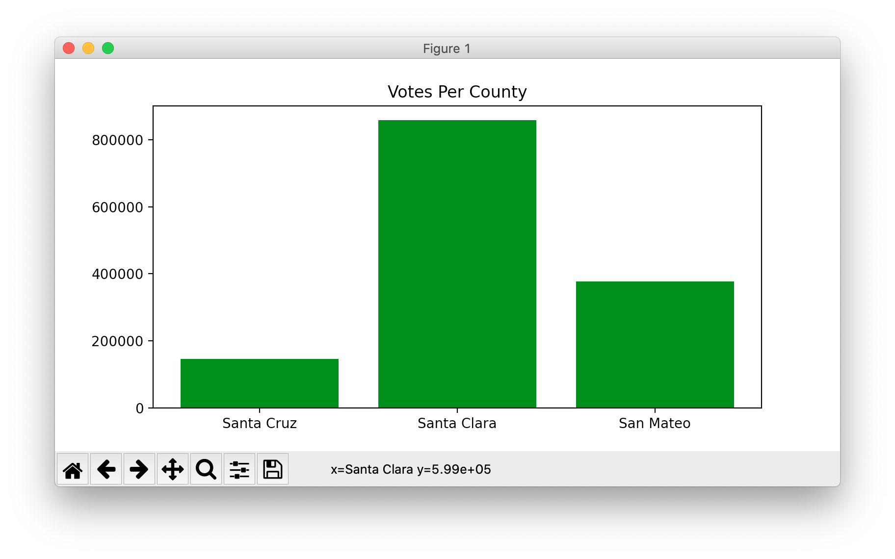
Here is the code run with the -ca1 flag. Computes the counts dict as above, then has some basic matplotlib calls to put the data on screen. You will need to be able to write code like this to make graphs.
def plot_ca1(filename):
    """Plot 3 counties - basic matplotlib"""
    votes = read_ca(filename)
    plt.figure(figsize=(8, 4))  # each unit is about 0.5 inch
    xs = ['Santa Cruz', 'Santa Clara', 'San Mateo']
    ys = [votes['Santa Cruz'], votes['Santa Clara'],
          votes['San Mateo']]
    plt.bar(xs, ys, color='green')
    plt.title('Votes Per County')
    # plt.xlabel('County')  # more titling on the graph
    # plt.ylabel('Votes')
    plt.show()
You can run with -ca1, runs the above code to make this chart. This is the sort of code you will need later.
$ python3 mystery.py -ca1 ca-2020-election.csv
Here is the matplotlib code for for the -ca2 option. This version plots 7 bay area counties. We don't want to have to manually type in the code to look up the value for each of the 7.
Instead, the code uses a comprehension to compute the ys value - look at the ys = .. line. It uses a comprehension: for each county in xs, look up its value in the counts dict. Your code can use the simpler -ca1 technique above, but this use of the comprehension does work very nicely.
def plot_ca2(filename):
    """Plot more ca counties, using comprehension"""
    votes = read_ca(filename)
    plt.figure(figsize=(8, 4))
    # Expand to 7 bay-area counties
    xs = ['Santa Clara', 'San Mateo',
          'Alameda', 'San Francisco',
          'Marin', 'Sonoma', 'Napa']
    # Instead of typing each county again,
    # comprehension pulls each county name
    # out of the xs variable - nice!
    ys = [votes[county] for county in xs]
    plt.bar(xs, ys, color='green')
    plt.title('Votes Per County')
    plt.show()
Run this to see the -ca2 data with
$ python3 mystery.py -ca2 ca-2020-election.csv
The function first_digits() takes in a list of numbers, computes a dict of how often each first digit appears, used in the matplotlib code below. The function output looks like this - here saying that the digit 4 appears 7 times, the digit 5 appears 3 times, and so on.
first_digits(nums) ->
  {4: 7, 5: 3, 7: 5, 2: 14, 9: 5, 1: 15, 8: 2, 6: 4, 3: 3}
Here is the code to draw 9 bars, for the digits 1, 2, 3, .. 9.
def plot_ca3(filename):
    """Plot first digits of all ca counties"""
    votes = read_ca(filename)
    nums = votes.values()
    counts = first_digits(nums)

    plt.figure(figsize=(8, 4))
    xs = ['1', '2', '3', '4', '5', '6', '7', '8', '9']
    plt.bar(xs, [counts[int(x)] for x in xs], color='green')
    plt.title('CA First Digits')
    plt.show()
$ python3 mystery.py -ca3 ca-2020-election.csv
That does not look random or uniform. What is going on here? Why are 1 and 2 so much more prevalent? Conspiracy to tamper with election data?
$ python3 mystery.py -tx tx-2020-election.csv
hmmm again. This conspiracy is widespread!
Quote: The most exciting phrase to hear in science, the one that heralds new discoveries, is not "Eureka!" (I found it!) but "That’s funny ..." - Isaac Asimov
$ python3 mystery.py -potato potato-production.csv
Hmm. Looks just like the Texas data. This conspiracy is everywhere!