Linguistics 278 class 8 and assignment 5
Introduction to Pandas
This introduction is mostly borrowed from a pandas cookbook by Julia Evans. So, she deserves most of the credit. I made things a bit more streamlined for class, updated some things for Python 3 and more recent versions of Pandas/matplotlib, and added a simple linguistic example at the end.
The main example here isn't a linguistics example. Maybe that'll be a refreshing change for the people in the class who aren't linguists?
Comment: What you have to do here is in one sense very easy. You'll mainly just be writing a line or two of Python using Pandas. But unfortunately, in another way it's very hard. It's just hard to understand and to work out how to use a big complex library like Pandas. That's just true, and everyone finds it that way until they get used to the library. But libraries are useful, so it's a good skill to practice! Don't forget to look at the documentation and for helpful examples on Google.
1. Getting set up
If you're going to do stuff with data and plots in Python – that is, be a data scientist – there's pretty much a standard recipe of stuff to do at the beginning … setting up iPython notebook for matplotlib and then importing the plotting and numerics and data analysis libraries. So let's do that first. There are conventionalized short names for these libraries that almost everyone uses…. So you should use them too.
# The usual preamble
%matplotlib notebook

import numpy as np
import pandas as pd
import matplotlib.pyplot as plt

# Make the plots a bit prettier (optional)
plt.style.use('ggplot')
For the exercise, we're going to use a dataset that is a subset of the 311 service requests that are available from NYC Open Data. It can act as our example of "big data". It has 110,000 service requests!
The service requests are available as a CSV file. You saw an example of a CSV file in the last question (Q10) of Assignment 1 (!). CSV files are a commonly used simple textual data format, commonly used with spreadsheets (Excel, etc.) and statistical packages (R, etc.). And also with Pandas. A data record is a line. Fields in the line are separated by commas. If the field contains a comma or just if you feel like it, you can quote a field value with double quotes. If you need to put a double quote inside a quoted field you can escape it with \". There are (unfortunately) a number of variants of CSV files in use, but that's the basic idea. Pandas provides an easy method for reading CSV files, called read_csv.
Now that we know about relative file paths, we can have the data in a data subdirectory. Functions/methods like open() or read_csv() actually take a file path (relative or absolute). We'd just kept things simple up until now by always having the data files in the same folder as our IPython Notebook. But once you start doing more complex things, you may well want to organize your data in separate folders.
complaints = pd.read_csv('data/311-service-requests.csv')
Ouch, you will have gotten an error like "DtypeWarning: Columns (8) have mixed types". This means that it's encountered a problem reading in our data. In this case it almost certainly means that it has columns where some of the entries are strings and some are integers.
For now we're going to ignore it and hope we don't run into a problem, but we need to investigate this warning. We talk about cleaning data later on. If you count the columns (starting from 0!, not counting the index at the beginning!), you find that the problematic column is "Incident Zip". We'll look at fixing that in section 6 below.
2. What's in this data?
When you print a large dataframe, it will only show you a few rows from the top and the bottom. That's meant to be helpful!
complaints
Pandas has 2 central data structures: Series, which are a one dimensional set of values, like a list (this isn't much use by itself, but appears when you select stuff from the other central data structure) and Dataframes, which are like the above (and which are really useful). A Dataframe is like a table of data. There are a whole set of data items, which are the rows, and then each data item has a set of attributes stored in a column. Each column has a name, and stores data of a particular type. Another special attribute of DataFrames is that they support the idea of a missing value, usually referred to as "N/A" or "na" (not available). This is again common to various statistics packages. Missing values are a fact of experimental life, and it is useful to have a package that considers the possibility of missing values.
3. Selecting columns and rows
To select a column, we index with the name of the column, like this, just as for an array:
complaints['Complaint Type']
To get the first 5 rows of a dataframe, we can use a slice: df[:5], just like we've learned about.
This is a great way to get a sense for what kind of information is in the dataframe – take a minute to look at the contents and get a feel for this dataset.
complaints[:5]
We can combine these to get the first 5 rows of a column:
complaints['Complaint Type'][:5]
And there's some magic going on! It just figures out whether you're talking rows or columns and indices or labels. You can specify them in either order. That still seems a little freaky to me!
complaints[:5]['Complaint Type']
If you want to avoid magic, you can with the .loc and .iloc attributes. The former is for label-based indexing and the latter is for positional indexing (e.g., row number). For example, here's the 100th data item. (This is also a way to see what all the columns are!)
complaints.iloc[100]
What if we just want to know the complaint type and the borough, but not the rest of the information? Pandas makes it really easy to select a subset of the columns: just index with list of columns you want.
complaints[['Complaint Type', 'Borough']]
That showed us a summary, and then we can look at the first 10 rows:
complaints[['Complaint Type', 'Borough']][:10]
But, wait, what are those double square brackets about? This is where it gets a bit tricky. If you use single square brackets, then you can specify a slice to select rows or a column name to select a column, and then you get back a Series. If you want to get multiple columns, you need a List (which I create with the inner square brackets) and then if you index with a List (indexing with the outer square brackets) you get back a Dataframe with multiple columns….
4. What complaints do people in New York have?
This is a really easy question to answer! There's a .value_counts() method that we can use. It makes a table with the counts of each value of a field.
complaints['Complaint Type'].value_counts()
There are a lot of cold people!
If we just wanted the top 10 most common complaints, we can do this:
complaint_counts = complaints['Complaint Type'].value_counts()
complaint_counts[:10]
But it gets better! We can plot them!
complaint_counts[:10].plot(kind='bar')
Q1: Find out what agencies complaints were filed with (the Agency column) and how many to each.
# Your code here
5. People who have noise complaints
Let's explore which borough has the most noise complaints. To get the sidewalk noise complaints, we need to find the rows where the "Complaint Type" column is "Noise - Street/Sidewalk". I'll show you how to do that, and then explain what's going on.
noise_complaints_sidewalk = complaints[complaints['Complaint Type'] == "Noise - Street/Sidewalk"]
noise_complaints_sidewalk[:3]
If you look at noise_complaints_sidewalk, you'll see that this worked, and it only contains complaints with the right complaint type. But how does this work? Let's deconstruct it into two pieces
complaints['Complaint Type'] == "Noise - Street/Sidewalk"
This is a big array of Trues and Falses, one for each row in our dataframe. When we index our dataframe with this array, we get just the rows where our boolean array evaluated to True. It's important to note that for row filtering by a boolean array the length of our dataframe's index must be the same length as the boolean array used for filtering.
You can also combine more than one condition with the & operator like this:
is_noise = complaints['Complaint Type'] == "Noise - Street/Sidewalk"
in_brooklyn = complaints['Borough'] == "BROOKLYN"
complaints[is_noise & in_brooklyn][:5]
Or if we just wanted a few columns:
complaints[is_noise & in_brooklyn][['Complaint Type', 'Borough', 'Created Date', 'Descriptor']][:10]
Q2. Find out which values the Descriptor column can have when the Complaint Type is "Noise - Street/Sidewalk"
# Code here
But, wait, if you looked at the statistics above, there were several types of noise complaints! If we wanted all kinds of noise complaints, we need to find more stuff. But we know Python, we can write a boolean condition for anything!
Almost, but there's still a bit to learn. When you get a column, it's a Series, and you can't just call string methods on a Series. But you can access the .str attribute, which provides methods that considerably mirror the methods of a str (but apply them to a whole Series at once).
You can match with regular expressions, but there are actually also string methods for exact initial and final subsequences of a string: str.startswith(prefix) and str.endswith(suffix), which you can also use here with str. Write something that gets all noise complaints. You can find out more about what you can do in the documentation
is_parking = complaints['Complaint Type'].str.contains("Parking")
complaints[is_parking]['Complaint Type'].value_counts()
You can match with regular expressions, but there are actually also string methods for exact initial and final subsequences of a string: str.startswith(prefix) and str.endswith(suffix), which you can also use here with str to find all noise complaints.
Q3. Write something that gets all noise complaints. You can find out more about what you can do with str fields in the documentation
# Write your code here
6. Which borough has the most noise complaints
Let's work it out just for street/sidewalk noise.
is_noise = complaints['Complaint Type'] == "Noise - Street/Sidewalk"
noise_complaints = complaints[is_noise]
noise_complaints['Borough'].value_counts()
It's Manhattan! But what if we wanted to divide by the total number of complaints in each borough, to make it make a bit more sense – giving the rate of noise complaints? That would be easy too:
noise_complaint_counts = noise_complaints['Borough'].value_counts()
complaint_counts = complaints['Borough'].value_counts()
noise_complaint_counts / complaint_counts
Let's plot the rate of sidewalk noise complaints:
(noise_complaint_counts / complaint_counts).plot(kind='bar')
So Manhattan really does spend more of its time complaining more about sidewalk noise than the other boroughs! Neat.
Q4. What if we now do all kinds of noise complaints? Do you get the same picture?
# Write code to get all noise complaints
# Write a line to get the counts by borough
# Write code to normalize by all types of complaints per borough
# Write code to plot the results
Do the same results still hold? Is noise a problem in Manhattan in general?
Answer:
6. Dealing with messy data
Usually, when you grab some data, it isn't clean. It has problems.
We're going to look at a few columns here. I know already that there are some problems with the zip code, so let's look at that first.
To get a sense for whether a column has problems, I usually use .unique() to look at all its values. If it's a numeric column, I'll instead plot a histogram to get a sense of the distribution.
When we look at the unique values in "Incident Zip", it quickly becomes clear that this is a mess.
Some of the problems:
- Some have been parsed as strings, and some as floats
- Some of the zip codes are
29616-0759or83 - There are some N/A values that pandas didn't recognize, like 'N/A' and 'NO CLUE'
What we can do:
- Normalize 'N/A' and 'NO CLUE' into regular nan values
- Look at what's up with the 83, and decide what to do
- Make everything strings
complaints['Incident Zip'].unique()
We can pass a na_values option to pd.read_csv to clean this up a little bit. We also specify that the type of Incident Zip is a string, not a float.
na_values = ['NO CLUE', 'N/A', '0', '000000']
complaints = pd.read_csv('data/311-service-requests.csv', na_values=na_values, dtype={'Incident Zip': str})
complaints['Incident Zip'].unique()
There are still a few items we might not want to deal with. Just a few people know their ZIP+4 codes! (The ones with the dash in them.) Note the special bit at the end of fillna(False). Some rows are missing their ZIP (it's blank). If I try to run the function without this last bit, it will error out in the second selection line, but by changing he missing values to false, those rows will just be ignored.
rows_with_dashes = complaints['Incident Zip'].str.contains('-').fillna(False)
complaints[rows_with_dashes]
Hmm…. Just 5 people out of 110,000 know their ZIP+4. Let's just truncate them to regular old 5 digit ZIP codes:
complaints['Incident Zip'] = complaints['Incident Zip'].str.slice(0, 5)
Fixed!
We got rid of some bad values while reading the file, but there is still a ZIP of 00000, which isn't valid.
complaints[complaints['Incident Zip'] == '00000']
We could just read the data again, adding in one more thing to na_values, or we could be clever and know that Pandas uses the numeric nan to represent a missing value, and just change it to that!
Remember: .loc: This attribute explicitly allows selection on each axis by either a boolean array or a label. .iloc: This attribute allows selection on each axis by an integer index, or again by a boolean array.
zero_zips = complaints['Incident Zip'] == '00000'
complaints.loc[zero_zips, 'Incident Zip'] = np.nan
unique_zips = complaints['Incident Zip'].astype(str).unique()
unique_zips.sort()
unique_zips
Why do I need the .astype(str)? Well, Pandas uses the numeric nan (not a number - an invalid number, like if you calculate 0/0 without throwing an exception) to represent the missing data value. We have missing values in the data. sort complains if it tries to compare this funny number with a str. We could also have fixed this as before using the .fillna() method
# Try doing it using the fillna method
unique_zips = complaints['Incident Zip'].fillna('').unique()
unique_zips.sort()
unique_zips
What about that 00083? Is that a problem? Sort of. It turns out that it's a semi-fictious zip code for Central Park! Which incidents have that ZIP?
complaints[complaints['Incident Zip'] == '00083']
We might want to get rid of it too. Let's change it to 10024, which is what the cops use for Central Park
# Change the items with ZIP code 00083 to 10024
cp_zips = complaints['Incident Zip'] == '00083'
complaints.loc[cp_zips, 'Incident Zip'] = '10024'
complaints[complaints['Incident Zip'] == '10024']
This is getting better and better! But there's still something a bit weird here, though – I looked up 77056 on Google maps, and that's in Texas.
Let's take a closer look:
zips = complaints['Incident Zip']
# Let's say the zips starting with '0' and '1' are okay, for now. (this isn't actually true -- 13221 is in Syracuse, and why?)
is_close = zips.str.startswith('0') | zips.str.startswith('1')
# There are a bunch of NaNs, but we're not interested in them right now, so we'll say they're False
is_far = ~(is_close) & zips.notnull()
zips[is_far]
Where are these places? Well, there's also a City column in the data! What does it say?
complaints[is_far][['Incident Zip', 'Descriptor', 'City']].sort_values(by='Incident Zip')
Hmm…. It looks like a few New Yorkers might call the 311 Hotline to complain even when they're on vacation in San Diego!
What is the range of cities we find?
complaints['City'].str.upper().value_counts()
This process is quite typical of what really goes on in the world. It's a commonly quoted figure that data scientists spend most of their time cleaning data. Not doing "science".
7. More plots
We're about done for learning a little Pandas, but there's other fun stuff in this data. Latitudes and longitudes! Dates! So we may as well have a bit more fun plotting stuff…. The funny '.' aargument below gives you a dot plot.
plt.plot(complaints['Longitude'], complaints['Latitude'], '.', color="purple")
Does every zip code complain about the same things? Here's some code that does that. (It's a bit complex. I'm not sure if I fully understand it or not….
popular_zip_codes = complaints['Incident Zip'].value_counts()[:10].index
zipcode_incident_table = complaints.groupby(['Incident Zip', 'Complaint Type'])['Descriptor'].aggregate(len).unstack()
top_5_complaints = zipcode_incident_table.transpose()[popular_zip_codes]
normalized_complaints = top_5_complaints / top_5_complaints.sum()
normalized_complaints.dropna(how='any').sort_values(by='11226', ascending=False)[:5].transpose().plot(kind='bar')
8. More data analysis: groupby, aggregate and unstack
But the part of the above example that you should make sure you understand is the query below.
If you run it, it'll take a while to run. Be patient! It creates a very big table. It first groups by incident zip and reported-to agency, and then it counts the number of rows for each combination of those. It then unstacks the last groupby and makes that the columns! So we now have a zip code by agency table! Finally, most of the cells have no items and so Pandas would put the missing value na or NaN there. I change it to an empty string. I could also have changed it to a count of 0, which would have been better if I were doing numeric work later. You'll need to use techniques we've seen like some of groupby(), value_counts(), aggregate() and unstack() to do the rest of the homework below!
complaints.groupby(['Incident Zip', 'Agency']).aggregate(len).unstack().fillna('')
9. A linguistic example
Here's another, much smaller and simpler, data file for a linguistic example. This is the data that was used in Bresnan, Dingare, and Manning (2001). Here's most of the abstract of that paper:
The same categorical phenomena which are attributed to hard grammatical constraints in some languages continue to show up as functionally motivated statistical preferences in other languages, motivating a grammatical model that can account for soft constraints. The effects of a hierarchy of person on grammar, favoring people Local to the conversation (1st and 2nd person) over Non-local people (1st, 2nd person > 3rd person), are categorical in some languages, most famously in languages with inverse systems, but also in languages with person restrictions on passivization. In Lummi (Straits Salish, British Columbia), for example, the person of the subject argument cannot be lower than the person of a nonsubject argument. If this would happen in the active, passivization is obligatory; if it would happen in the passive, the active is obligatory (Jelinek and Demers 1983). These facts can be said to follow from the theory of harmonic alignment in OT: constraints favoring the harmonic association of prominent person (1st, 2nd) with prominent syntactic function (subject) are hypothesized to be present as subhierarchies of the grammars of all languages, but to vary in their effects across languages depending on their interactions with other constraints (Aissen 1999). There is a statistical reflection of these hierarchies in English. The same disharmonic person/argument associations (a 1/2 object when there is a 3 subject) which are avoided categorically in languages like Lummi by making passives either impossible or obligatory, are avoided in the SWITCHBOARD corpus of spoken English by either depressing or elevating the frequency of passives relative to actives.
In other words, we look at clauses involving canonical transitive (2 argument) verbs, both arguments being human, such as I nudged him. We refer to the doer as the agent and the person acted on as the patient. Our prediction is that there should be a soft preference disfavoring a 3rd person (he, she, it, they) subject when the other argument is 1st or 2nd person (I, me, you). English can always avoid this situation by passivizing the clause if the agent is 3rd person and the patient is 1st/2nd person, while using the active if the agent is 1st/2nd person and the patient is 3rd person.
Q5. The file is 'data/bdm-2001-data.csv'. Load it as a CSV file. And look at a few lines to get an idea of what is there.
# Load it as a CSV file
# Look at a few lines
Q6. Much simpler, huh? You can also get a summary of the contents of a Dataframe by using the .describe() method on it. Try that.
# Get a summary of the data frame
Q7. Now what we have is rows for individual clauses, but what we'd like here is counts for how often different configurations happened. To do that, we want to use groupby aggregation again, and to get the count of each of the configurations that occur. (There are 8 possible configurations, because there are 2 values for each of 3 fields. Try to do that with groupby(). Look back to the examples above, or look online for ideas as to how.
# Code
Q8. Two configurations actually don't occur in the data at all. Which are they? (There still isn't a categorical prohibition on these configurations in English; you can find examples in large text collections.)
The non-occurring configurations are:
Q9. Let's make a table showing the rate (percentage of times) passivization occurs for the four different configurations of active and passive. Your aim is to produce the below table but with the cells filled in with numbers.
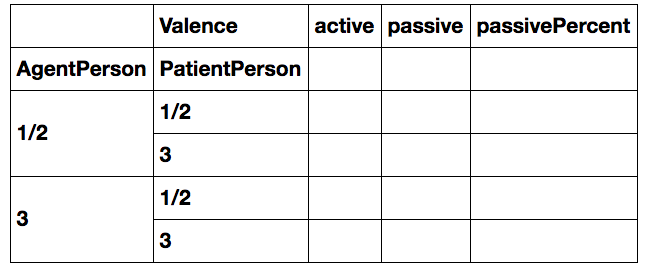
# Code to fill in such a table
Q10. Is the hypothesis confirmed? Is there a preference to use passivization (valence) to avoid having a 3rd person subject when the other argument is 1st/2nd person?
Answer:
# I'm sure to need this in class sometime!
plt.close("all")