For this project, you will bring the Baby Names data to life.
When Python is installed on a machine, it includes the venerable "TK" graphics systems via the "tkinter" module. It can create graphical windows, buttons etc. on screen - the graphical user interface (GUI). We provide the code that sets up the GUI. That code is not very interesting. TK is a very old system, so the code to set it up is kind of archaic too, but it works fine for our purposes. To learn modern GUI techniques, you could take CS108 or CS142. In this case, the functions you need to write are at the top of the file, and the provided TK functions are below.
The main() code is provided in babygraphics.py. The main() function calls your babynames.read_files() function to read in the names data. The challenge on this assignment is providing an interactive GUI for the baby data. Run the program from the command line in the usual way.
$ python3 babygraphics.py
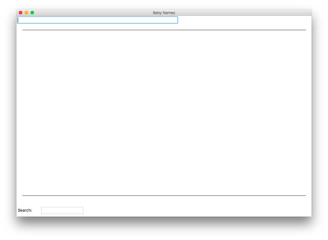
Without adding any code, running babygraphics.py should load the baby data, and display a largely empty window which waits for you to type something. The text field at the top of the window takes in names, and the text field at the bottom is for the search feature. The provided code takes care of setting up the GUI elements, and detecting when the return-key is typed to call your search and draw functions. Click in the search field at the bottom, type "arg" or "aa" and hit return. The provided handle_search() functions calls your babynames.search_names() function, and pastes the result into the window. Those functions were called to print output in the terminal for HW 6a. Here, the GUI code calls the exact same functions, but puts the output in the GUI.
Syntax: here is the key line in the provided handle_search() where it calls your search_names() function from HW6a:
    ...
    # Call the search_names function in babynames.py
    result = babynames.search_names(names, target)
    ...
Milestone search: you can run babygraphics and see the results of searches like "aa" and "arg" in the GUI.
Here are constants for the use in the babygraphics algorithms. The number of years of data is given by len(YEARS).
# Provided constants to load and draw the baby data
FILENAMES = ['baby-1900.txt', 'baby-1910.txt', 'baby-1920.txt', 'baby-1930.txt',
             'baby-1940.txt', 'baby-1950.txt', 'baby-1960.txt', 'baby-1970.txt',
             'baby-1980.txt', 'baby-1990.txt', 'baby-2000.txt', 'baby-2010.txt',
             'baby-2020.txt']

YEARS = [1900, 1910, 1920, 1930, 1940, 1950, 1960, 1970, 1980, 1990, 2000,
         2010, 2020]
SPACE = 20
COLORS = ['red', 'purple', 'green']
TEXT_DX = 2
LINE_WIDTH = 2
MAX_RANK = 1000
Look at the YEARS constant above. For each year there are actually two values your code might use - the int year itself, e.g. 1900 or 1910. For each of those years, there is also the year_index, indicating where that year is in the YEARS list, e.g. 0 or 1. It's easy to get those two related quantities mixed up in your code — a good place to use good variables names to keep things straight.
The draw_fixed() function draws the fixed lines and text behind the data lines. It is called once from main() to set up the window initially, and then again whenever the graph is re-drawn. When draw_fixed() runs, the canvas is some width/height in the window. The provided code retrieves those numbers from the canvas for use by the subsequent lines.
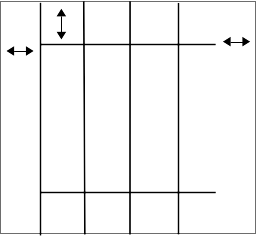
Draw the year grid as follows. All of these drawings are in black: The provided constant SPACE=20 defines an empty space which should be reserved at the 4 edges of the canvas. Draw a top horizontal line, SPACE pixels from the top, and starting SPACE pixels from the left edge and ending SPACE pixels before the right edge. Draw a bottom horizontal line SPACE pixels from the bottom edge, and SPACE from the left and right edges. We will not be picky about +/- 1 pixel coordinates for this assignment.
Here is a diagram of the line spacing for draw_fixed(). The outer edge of the canvas is shown as a rectangle, with the various lines drawn within it. Each double-arrow marks a distance of SPACE pixels.
In the GUI, the name text field is at the top of the window, and the canvas is a big rectangle below it. Then the search text field is at the bottom of the window below the canvas.
YEARS = [1900, 1910, 1920, 1930, 1940, 1950, 1960, 1970, 1980, 1990, 2000,
         2010, 2020]
The provided constant YEARS lists the int years to draw. Any function is free to read from constants like YEARS when needed. In draw_fixed(), draw a vertical "year" line for each year in YEARS. The first year line should be SPACE pixels from the left canvas edge. The year lines should touch the 2 horizontal lines, spaced out proportionately so each year line gets an equal amount of empty space to its right on the horizontal lines. Vertically, the year lines should extend all the way from the top of the canvas to its bottom.
The trickiest math here is computing the x value for each year index. Write code for the short helper function compute_x() to compute the x coordinate in the canvas for each year index: 0 (the first year), 1 (the second year), 2, .... len(YEARS)-1 (the last year). No loops or if-statements are required for this short function. There are a few spots in the program where you need to know what x values goes with each year index, so this helper function can be used in all those places. Doctests are not required.
def compute_x(width, year_index):
    """
    Given canvas width and year_index 0, 1, 2 .. into YEARS list,
    return the x value for the vertical line for that year.
    """
For drawing, we will use Python's built in "TK" drawing functions which are similar but not identical to the DrawCanvas functions we used earlier. The drawing functions truncate coordinates from float to int internally, so you should do your computations as float. The function to draw a black line in TK is:
canvas.create_line(x1, y1, x2, y2)
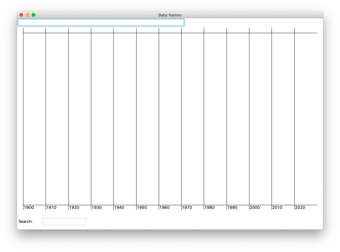
At a point TEXT_DX pixels to the right of the intersection of each vertical line with the lower horizontal line, draw the year string. The TK create_text() function shown below will draw the 'hi' string with its upper left corner at the given x/y. The constant tkinter.NW indicates that the x,y point is at the north-west corner relative to the text.
canvas.create_text(x, y , text='hi', anchor=tkinter.NW, fill='red')
The optional parameter fill='red' specifies a color other than the default black for the TK functions like create_line() and create_text().
By default, main() creates a window with a 1000 x 600 canvas in it. Try running main() like this to try different width/height numbers:
$ python3 babygraphics.py 800 400
Your line-drawing math should still look right for different width and height values. Note that if you specify a width of, say, 400, that will be the size of the canvas, but the window may be a wider number since it also needs space to the right of the search text field to display the search results. You should also be able to change temporarily, say, the SPACE constant to a value like 100, and your drawing should use the new value. (SPACE is a good example of a constant - a value which is used in several places. Defining it as a constant makes it easy to change, and the lines of code that use it remain consistent with each other.)
Milestone draw-fixed: your code can create all the fixed straight lines and year strings and work for various window widths and heights.
Ultimately, the draw_names() function should take in any number of names and draw all their data. The starter code for draw_names() works in a special "Jennifer" mode where it always draws the name "Jennifer" when you hit the return key with the cursor in the top text field (or some other single name you typed in there). This is a handy way to work on the draw_name() function without having to type a lot in the GUI. In a later step, you will upgrade draw_names() out of its always-Jennifer mode.
The names in the SSA data set all have an upper case character as their first character, e.g. 'Emily'. To shield the user from that detail, the provided code converts what the user types in, e.g. 'emily', to the SSA 'Emily' form before draw_names() is called. In this way, the user can type the names in without worrying about capitalization.
This is a helper function for the data drawing code. There is a problem when trying to draw the data for a name and year: some years have data and some do not. For example, in the Jennifer data, there's nothing in the years before 1940.
{1940: 690, 1950: 118, ...}
The drawing code is most straightforward if every year has a rank number to draw, without worrying about the details behind that rank number. Our solution is this: if a name does not have data for a particular year (e.g. 'Jennifer' in 1900), or if the name itself does not appear in the name dict at all, e.g. the name 'Xyz', then we'll say that the rank number to use is MAX_RANK.
Given a complication like this, the CS strategy is to wrap it up in a function. Write code for the compute_rank() helper function which isolates this issue — if a name and year have a rank number, return that number. Otherwise, return MAX_RANK. Doctests are provided.
def compute_rank(names, name, year):
    """
    Given names dict, name string, and int year.
    Return the best rank to use: the actual rank if
    that name+year exists in the data, or MAX_RANK
    if the name or year is not present.
    >>> # Tests provided, code TBD
    ...
Milestone compute-rank: best_rank() passes its tests.
To draw the data for a name like "Jennifer", for each year index, we need to figure the y value for that year_index. It's handy in the later stages to have a helper function for this y-computation.
To compute the y, first get the rank number using your helper. Work out a formula so when rank is 1 (the best possible rank), the y should be at the very top (covering the top horizontal line). If rank is MAX_RANK, the y should be at the very bottom (covering the bottom horizontal line). No loops or if-statements are required for this function. Instead of Doctests, we'll just see how it draws on screen in the next section.
def compute_y(names, name, height, year_index):
    """
    Given names dict, name string, canvas height, and
    year_index 0 1 2 ..., compute and return the y for
    the that name/year_index line endpoint.
    """
def draw_name(canvas, names, name, color):
The draw_name() function is the heart of the program — taking one name, and drawing its data across all the years. The draw_name() function has parameters for the names dict, name string, and color to use for the drawing.

Suppose the passed in name is 'Jennifer'. For every year, the code looks up the Jennifer rank for that year, and gets the x and y values for each year using the helper functions.
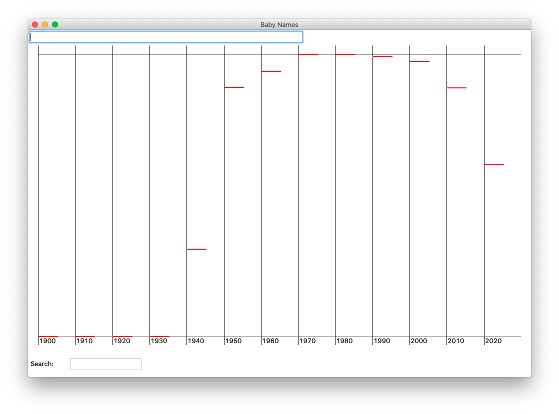
As a milestone, figure the x,y for each year for the given name, and as a temporary measure, draw a horizontal line starting at that x,y and extending rightwards 40 pixels (each x,y is a little dot in the drawing below). As mentioned above "Jennifer" is a nice example here, as the name hits both the min and the max possible ranks, something of an achievement for a single name. In effect, this code will test your compute_x() and compute_y() helpers by putting their results on screen.

The default TK create_line() draws a 1-pixel-wide line. For draw_name(), it looks better to draw the lines with a little more thickness. Use the constant LINE_WIDTH and the color parameter as shown below to draw a thick, colored line. The parameters to create_line() don't have great names in this context: "width" is the thickness of the line, and "fill" is its color. The line of code below draws in red, and you can fix it later to use the right color.
canvas.create_line(x1, y1, x2, y2, width=LINE_WIDTH, fill='red')
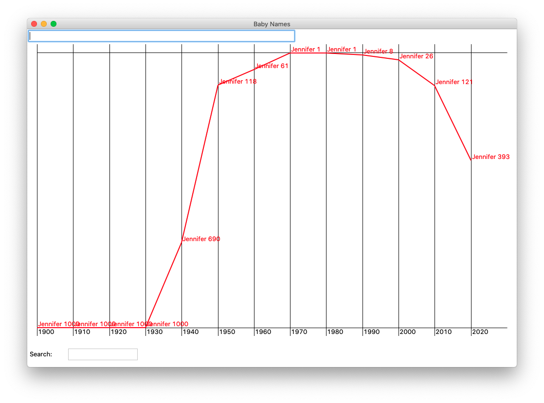
Here's a picture of the Jennifer data with the 40-pixel lines. Hitting the return key with the cursor in the input field should call draw_name() this way. Jennifer has no data in 1900, and is #1 in 1970. You can scroll down to the later stages to see the full Jennifer data curve.
You can type a different name in the top text field, and draw_name() will be called with that name, so you can try different names to see your x,y code at work.
Milestone draw-name-1: for a name, your code can loop over all the years, figuring out the right x,y, for every year and draw the 40 pixel line.
With the x,y working for every year, draw the name and rank as a string, e.g. 'Jennifer 690', TEXT_DX pixels to the right of each year/rank point. The call to canvas.create_text(..) is the same as before, except using the constant tkinter.SW to position the text above and to the right of the x,y point.

Drawing in all the lines is an algorithmic puzzle. For N years of data, there are N-1 lines to draw, connecting the x,y of each year, to the x,y of the previous year, skipping the first year which does not have a previous year. Either of the following techniques is fine.
Approach 1: for each year index other than the first, call the helpers to get the x,y of the previous year, and then draw a line from the current x,y to the previous year x,y. This is a good technique for this homework, leveraging the helpers to access both the current and previous year x,y.
Approach 2: Rather than re-compute the x,y when needed, use the "previous" pattern to remember the x,y across iterations. So in iteration i of the loop, the previous pattern gives access to the x,y from iteration i - 1. For each point except the first, draw a line from the current x,y back to the previous x,y. This is also a good technique for the homework, being a little clever about not re-computing things, but also a little tricky.
Here is the Jennifer output with all the text and lines working:
Milestone draw-name-2: for one name, the code loops over all the years, drawing in all the lines and text labels.
The last step is fixing draw_names() to get out of its "Jennifer" dev mode. Delete the Jennifer dev-mode code from draw_names().
The "lookups" parameter is a list of name strings to process, e.g. ['Jennifer', 'Miguel', 'Anna']. The provided code builds the lookups from whatever the user types in the top text field, converting the first char of each word to uppercase. Within the text field, the user may separate the names by spaces, and commas also work. At the your-code-here mark, write code to draw all of the name strings in the lookups list, calling your draw_name() function once for each name.
The provided constant COLORS is a list of 3 color names. Draw the name at index 0 with the color at index 0. Draw name at index 1 with color 1, wrapping around to color 0 after all the colors are used, like this:
name_index   color_index
0             0
1             1
2             2
3             0
4             1
5             2
6             0
7             1
...
Use the modulo % operator to get the wrap-around effect. Do not use the number 3 in your code, use len(COLORS), so if you add a 4th color in the COLORS, the drawing will automatically use it (similar to using the constant SPACE in the drawing code instead of the number 20).
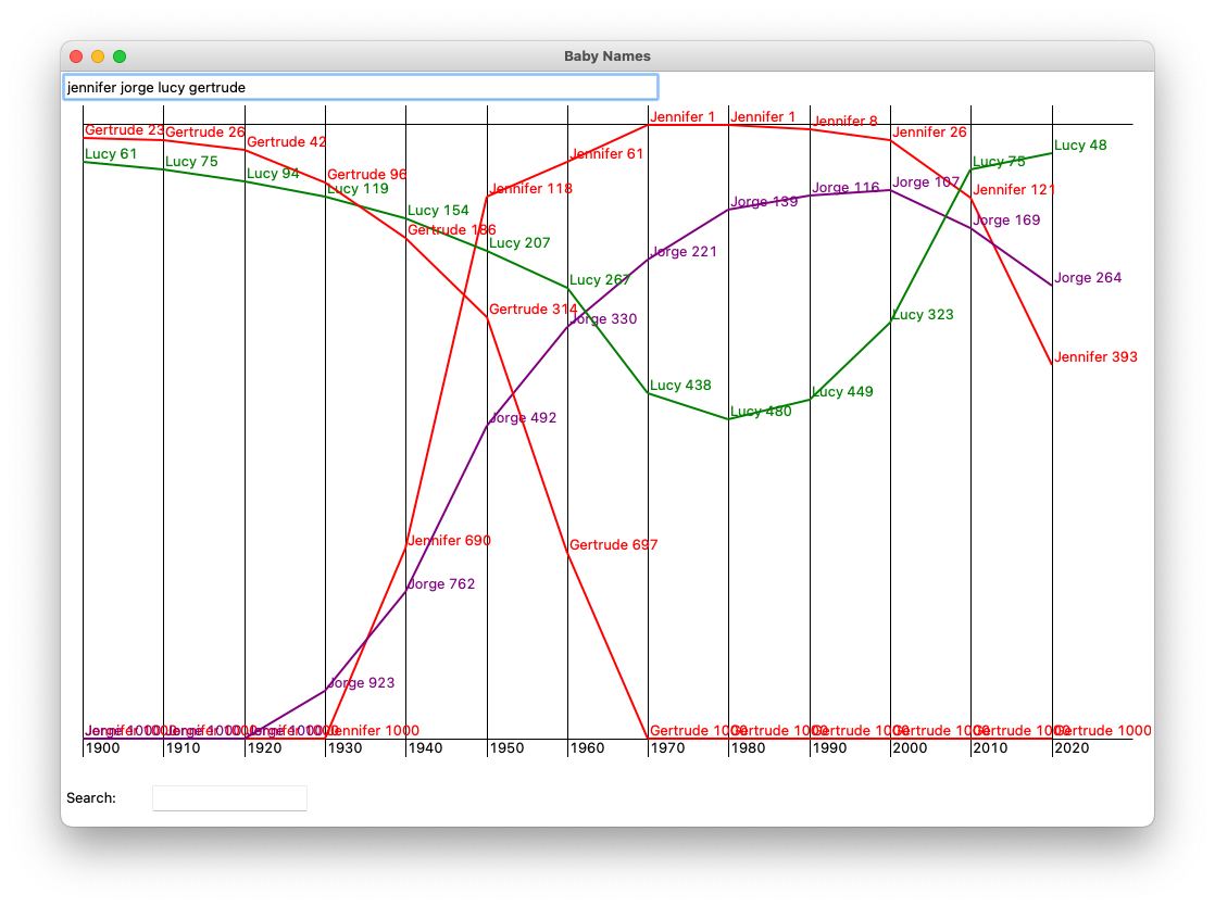
Once the code is drawing all the lookups properly, you can take the program for a spin. "Jennifer" is a good test of course, but now we can layer on the data for Jorge and Lucy and Gertrude. Note in screenshot below that Gertrude is drawn in red, since it is at index 3, getting the wrap-around effect.
Isn't "Chad" like some internet insult for something? Well check out Chad's graph. Compare it to Hazel. I don't think Madge is coming back either. Use your search feature to find more names. What names can you think of that have "haz" or "enz" in them? Try it in the search field at the bottom to see. Search for "marg" to see the many variations on Margaret. Try the names of your parents and grandparents and their friends. Many will be out of fashion, but some, like Emily, will have amazing comebacks.
Once it's drawing everything nicely - congratulations - you've built a complete end-to-end program: parsing the raw data, organizing it in a dict, and presenting it in an interactive GUI. With your code cleaned up, please turn in the two files babynames.py and babygraphics.py on Paperless.
Nick Parlante created the Baby Names assignment around 2004 for the then new Java version of CS106A and later brought it over to Python/TK. In the Python version, there is greater use of decomposition to divide the complex drawing algorithm into manageable pieces. The original inspiration came from the article Where Have All The Lisas Gone about how parents choose baby names, often wanting a name that is rare but not too rare.
The data has been organized in a few different ways over the years, but it's always combined the algorithmic challenge of complex name/year data at one level, and then the loop/drawing logic above it to bring the data to the screen. The data set is large and fun, and that helps make the assignment fun too. The assignment was subsequently selected for the Nifty Assignments archive and has been adopted by many schools.