Today: del, matplotlib, jupyter notebooks, numpy
CS106A covers the most important features for programming. Today we'll look at Python a few Python features you might want to use in the future. These are not on the final!
is, Not Same as ==is None1. Say we have a word variable. The following if-statement will work perfectly for CS106A, and you probably wrote it that way before, and it's fine and we will never mark off for it.
if word == None:       # Works fine, not PEP8
    print('Nada')
2. However, there is a very old rule in PEP8 that comparisons to the value None should be written with the is operator. This is an awkward rule, but we are stuck with it. You may have noticed PyCharm complaining about the above form, so you can write it as follows and it works correctly and is PEP8:
if word is None:       # Works fine, PEP8
    print('Nada')


if word is not None:   # "is not" variant
    print('Not Nada')
Very important limitation:
3. The is operator is similar to ==, but actually does something different for most data types, like strings and ints and lists. For the value None, the is operator is reliable. Therefore, the rule is:
Never use the is operator for values other than None.
Never, never, never, never.
Only use is with None as above. If you use it with other values, it will lead to horrific, weekend-ruining bugs.
See Python copy/is chapter for the details.
>>> nums = [1, 2, 3, 4, 5, 6]
>>> [n + 10 for n in nums]
[11, 12, 13, 14, 15, 16]
>>> [abs(n - 3) for n in nums]
[2, 1, 0, 1, 2, 3]
>>> [str(n) + '!!' for n in nums]
['1!!', '2!!', '3!!', '4!!', '5!!', '6!!']
Matplotlib is an extremely capable and popular, open-source Python module for producing visualizations of data. Install it with "pip" like this:
$ python3 -m pip install matplotlib
Matplotlib is super popular with researches and media for generating visualizations. The number of features and variations available Matplotlib is a little dizzying. We will just scratch the surface here, so you get a feel for what's there.
See the official matplotlib.org and here is a popular tutorial (with tons of ads!): Matplotlib Tutorial
For this lecture example, we'll just use the few matplotlib features shown below.
At top of file, have the following import form. This sets up "plt" as the name to be used in the file. This is a standard import for matplotlib, see it in examples etc, so we'll use it too.
# standard import line .. 'plt' is idiomatic here
import matplotlib.pyplot as plt
Download to get started
mystery-data.zip. There's a lot of real data in here we can graph.
The file "mystery-plot.py" is complete; we'll just play with it to experiment with matplotlib, and it is working example matplotlib code.
Data source: there's a nicely organized 2020 data set - graphics at the New York Times and other things you've seen are built from this data. It's also huge and complicated! The California and Texas data sets below are from this url.
The file ca-2020-election.csv looks like this: (you can click on it from within Pycharm to see it). There are more than 70,000 lines of data in here, with data for each voting precinct in California.
COUNTY,FIPS,RGPREC_KEY,ELECTION,TYPE,RGPREC,TOTREG_R,DEM,REP,AIP,PAF,MSC,LIB,NLP,GRN...
25,06049,0604902001,g20,V,02001,96,22,41,1,0,1,2,0,0,0,29,40,56,3,0,2,0,0,1,0,0,0,0,0,0,0...
25,06049,0604904001,g20,V,04001,111,25,61,6,0,0,1,0,0,0,18,58,53,0,2,1,1,0,0,0,0,0,0,2,0,0...
25,06049,0604906001,g20,V,06001,365,101,184,16,2,0,2,0,4,0,56,166,199,5,10,2,1,5,4,3,1,0,0,..
..
How to parse this? No problem! (1) for line in f, (2) line.split(','). See the function read_ca() which parses the above, computing totals per county in a dict which is returned.
Run like this to see the dict computed by read_ca(), where the county name is the key, and the total votes in that county is the value.
$ python3 mystery-plotmystery-plot.py -ca ca-2020-election.csv
{'Modoc': 4349, 'Madera': 53889, 'Napa': 72700, 'Sonoma': 268569, 'Merced': 90482, 'Kern': 298938, 'San Joaquin': 281988, 'San Benito': 28724, 'Stanislaus': 211971, 'Ventura': 427164, 'Santa Cruz': 146024, ...
$
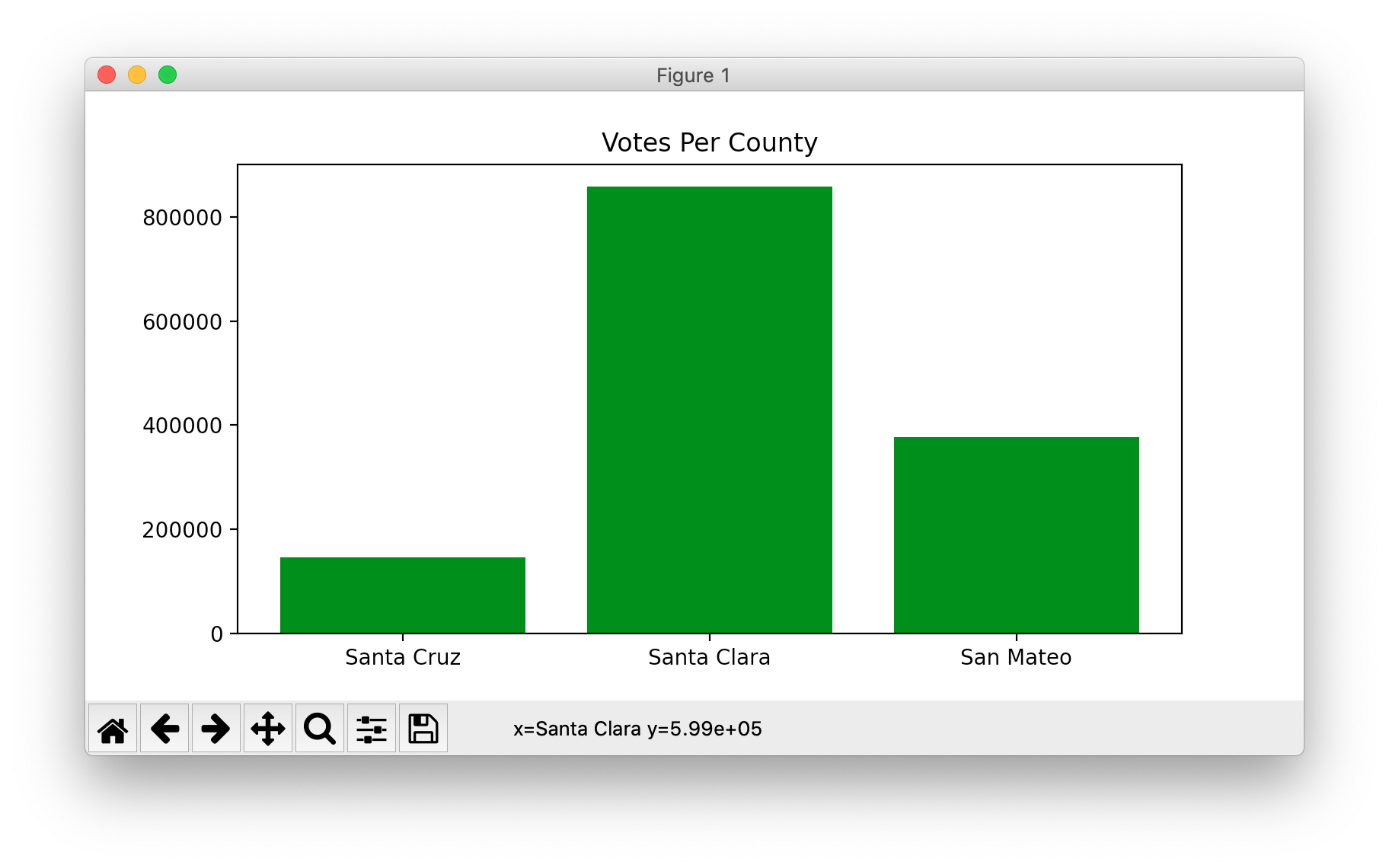
Here is the code run with the -ca1 flag. Computes the counts dict as above, then has some basic matplotlib calls to put the data on screen. This is a basic example of pulling in some data in Python, and then calling matplotlib to graph it.
def plot_ca1(filename):
    """Plot 3 counties - basic matplotlib"""
    votes = read_ca(filename)
    plt.figure(figsize=(8, 4))  # each unit is about 0.5 inch
    xs = ['Santa Cruz', 'Santa Clara', 'San Mateo']
    ys = [votes['Santa Cruz'], votes['Santa Clara'],
          votes['San Mateo']]
    plt.bar(xs, ys, color='green')
    plt.title('Votes Per County')
    # plt.xlabel('County')  # more titling on the graph
    # plt.ylabel('Votes')
    plt.show()
You can run with -ca1, runs the above code to make this chart. This is the sort of code you will need later.
$ python3 mystery-plot.py -ca1 ca-2020-election.csv
Here is the matplotlib code for the -ca2 option. This version plots 7 bay area counties. We don't want to have to manually type in the code to look up the value for each of the 7.
Instead, the code uses a comprehension to compute the ys value - look at the ys = .. line. It uses a comprehension: for each county in xs, look up its value in the counts dict. This is short, and also avoids the sort of error you might make, manually trying to have the xs and ys lists be in the same order.
def plot_ca2(filename):
    """Plot more ca counties, using comprehension"""
    votes = read_ca(filename)
    plt.figure(figsize=(8, 4))
    # Expand to 7 bay-area counties
    xs = ['Santa Clara', 'San Mateo',
          'Alameda', 'San Francisco',
          'Marin', 'Sonoma', 'Napa']
    # Instead of typing each county again,
    # comprehension pulls each county name
    # out of the xs variable - nice!
    ys = [votes[county] for county in xs]
    plt.bar(xs, ys, color='green')
    plt.title('Votes Per County')
    plt.show()
Run this to see the -ca2 data with
$ python3 mystery-plot.py -ca2 ca-2020-election.csv
The function first_digits() takes in a list of numbers, computes a dict of how often each first digit appears, used in the matplotlib code below. The function output looks like this - here saying that the digit 4 appears 7 times, the digit 5 appears 3 times, and so on.
first_digits(nums) ->
  {4: 7, 5: 3, 7: 5, 2: 14, 9: 5, 1: 15, 8: 2, 6: 4, 3: 3}
Here is the code to draw 9 bars, for the digits 1, 2, 3, .. 9.
def plot_ca3(filename):
    """Plot first digits of all ca counties"""
    votes = read_ca(filename)
    nums = votes.values()
    counts = first_digits(nums)

    plt.figure(figsize=(8, 4))
    xs = ['1', '2', '3', '4', '5', '6', '7', '8', '9']
    plt.bar(xs, [counts[int(x)] for x in xs], color='green')
    plt.title('CA First Digits')
    plt.show()
$ python3 mystery-plot.py -ca3 ca-2020-election.csv
That does not look random or uniform. What is going on here? Why are 1 and 2 so much more prevalent? Conspiracy to tamper with election data?
$ python3 mystery-plot.py -tx tx-2020-election.csv
hmmm again. This conspiracy is widespread!
Quote: The most exciting phrase to hear in science, the one that heralds new discoveries, is not "Eureka!" (I found it!) but "That’s funny ..." - Isaac Asimov
$ python3 mystery-plot.py -potato potato-production.csv
Hmm. Looks just like the Texas data. This conspiracy is truly everywhere!
This command will install both jupyter and matplotlib
$ python3 -m pip install jupyter matplotlib
$ jupyter notebook
This example starts with delay data for hours 0-23 of every day for a year. Process it to make a graph showing average delay for each hour of the day. Some of the support code is in traffic.py, and we call its functions from within the notebook.
With notebook form, you are kind of "live" playing with calling your functions, fitting the data into graphs, reacting to what you see in the moment. You can publish your analysis and output as a noteobook, essentially the mechanism to create to create the work - invites iteration and study.
A Jupyter notebook is interactive, showing the steps to follow with the output of each step.
The code in the notebook makes simple matplotlib calls to insert some graphs.
# standard import line .. 'plt' is idiomatic here
import matplotlib.pyplot as plt

# 1. plot 1-d list of values. plot() uses lists
plt.plot([5, 13, 2, 7])
plt.show()


# 2. Provide both x-values and y-values lists to plot() - a common pattern
# specify color, titling
plt.title('Some Words Here')
# plot() pattern: plot( [ x-values ], [ y-values] )
plt.plot([1, 2, 3, 4], [5, 13, 2, 7], color='red')
plt.show()

$ python3 -m pip install numpy
This example creates a numpy array. Look at its dimensions, compute "sum" a couple ways. numpy supports common numerical patterns, including the vector/matrix operations of linear algebra.
>>> import numpy as np
>>>
>>>
>>> a = np.array([[1, 2, 3],     # Create 2-d array
...               [4, 5, 6]])
>>>
>>> # len 1st dimension = 2, len of 2nd dim = 3
>>> a.shape
(2, 3)
>>>
>>> a.sum()         # sum of whole thing
np.int64(21)
>>> a.sum(axis=0)   # vector of sums, taking out axis 0
array([5, 7, 9])
>>> a.sum(axis=1)   # vector of sums, taking out axis 1
array([ 6, 15])
Demo copy: import numpy as np; a = np.array([[1, 2, 3], [4, 5, 6]])
Then try: a.sum(axis=0)
We may get this far.
del - Delete - The Spell of UnmakingThe del operator in Python is unusual operator. You will never need del in CS106A, so we'll just a take a glance at it. The del operator is followed by a reference to a Python data structure, and it deletes or unmakes it.
1. del d[key] - deletes key from a dict
2. del lst[index] - deletes the element at index from a list, shifting elements down as needed. Works with slices to remove whole sections from a list.
3. del x - deletes the binding of a variable, so it is no longer defined.
This reminds me of the works of author Ursula Le Guin, where there is a balance between the powers of making and unmaking. The del operator reminiscent of unmaking.
>>> d = {'a': 'alpha', 'g': 'gamma', 'b': 'beta'}
>>>
>>> d['b']
'beta'
>>> del d['b']
>>> d
{'a': 'alpha', 'g': 'gamma'}
>>>
>>> lst = ['a', 'b', 'c', 'd']
>>> lst[0]
'a'
>>> del lst[0]
>>> lst
['b', 'c', 'd']
>>>
>>> x = 6
>>> x
6
>>> del x
>>> x
NameError: name 'x' is not defined