1. Introduction
Large organizations generate lot of internal data, and also consume
data produced by third party providers. Many data providers obtain
their data by processing unstructured sources, and invest significant
effort in providing it in a structured form for use by others. To make
an effective use of such external data, it must be related to company's
internal data. Such data integration enables many popular use cases
such as 360 view of a customer, fraud detection, risk assessment, loan
approval etc. For this chapter, we will discuss the problem of
creating a knowledge graph by integrating the data available from
structured sources. We will consider the problem of extracting data
from unstructured data sources in the next chapter.
When combining data from multiple sources into a knowledge graph,
we can undertake some upfront design of schema as we discussed in
the previous chapter. We can also begin with no schema as it is
straightforward to load external data as triples into a knowledge
graph. The design of the initial schema is typically driven by the
specific business use case that one wishes to address. To the degree
such an initial schema exists, we must determine how the data
elements from a new data source should be added to the knowledge
graph. This is usually known as the schema mapping
problem. In addition to relating the schemas of the two sources, we
also must deal with the possibility that an entity in the
incoming data (e.g., a Company) may already exist in our knowledge
graph. The problem of inferring if the two entities in the data may
be the same real world entity is known as the record
linkage problem. The record linkage problem also arises when
third party data providers send new data feeds, and our knowledge
graph must be kept up-to-date with the new data feed.
In this chapter, we will discuss the current approaches for
addressing the schema mapping and the record linkage problems. We
will outline the state-of-the-art algorithms, and discuss their
effectiveness on the current industry problems.
2. Schema Mapping
Schema mapping assumes the existence of a schema which will be used
for storing new data coming from another source. Schema mapping then
defines which relations and attributes in the input database
corresponds to which properties and relations in the knowledge
graph. There exist techniques for bootstrapping schema mappings. The
bootstrapped schema mappings can be post corrected through human
intervention.
We will begin our discussion on schema mapping by outlining some of
the challenges and arguing that one should be prepared for the
eventuality that this process will be largely manual and
labor-intensive. We then describe an approach for specifying
mappings between the schema of the input source and the schema of
the knowledge graph. We will conclude the section by considering
some of the techniques that can be used to bootstrap schema mapping.
2.1 Challenges in Schema Mapping
The main challenges in automating schema mapping are: (1) difficult
to understand schema (2) complexity of mappings, and (3) lack of
training data available. We next discuss these
challenges in more detail.
Commercial relational database schemas can be huge consisting of
thousands of relations and tens of thousands of attributes. Sometimes,
the relation and attribute names do not have semantics (e.g.,
segment1, segment2) which do not lend themseves to any realistic
automated prediction of the mappings.
The mappings between the input schema and the schema in the
knowledge graph is not always simple one-to-one mapping. Mappings may
involve calculations, applying business logic, and taking into account
special rules for handling situations such as missing values. It
becomes a tall order to expect any automatic process to infer such
complex mappings.
Finally, many automated mapping solutions rely on machine learning
techniques which require large amount of training data to function
effectively. As the schema information, by definition, is much smaller
than the data itself, it is unrealistic to expect that we will ever
have large number of schema mappings available against which a mapping
algorithm could be trained.
2.2 Specifying Schema Mapping
In this section, we will consider one possible approach to specify
mappings between input data sources and a target knowledge graph
schema. We will take an example in the domain of cookware. We can imagine
different vendors providing products which an E-commerce site may wish
to aggregate and advertise to its customers. We will consider two
example sources, and then introduce the schema of the knowledge graph
to which we will define mappings.
We show below some sample data from the first data source in a
relational table called cookware. It has four
attributes: name, type, material,
and price.
| cookware |
|---|
| name | type | material | price |
|---|
| c01 | skillet | cast iron | 50 |
| c02 | saucepan | steel | 40 |
| c03 | skillet | steel | 30 |
| c04 | saucepan | aluminium | 20 |
|
The second database shown below lists the products of a
manufacturer. In this case, there are multiple tables, one for each
product attribute. The kind table specifies the type of each
product. The base table specifies whether each product is
made from a corrosible metal (aluminum or stainless), a noncorrosible
metal (iron or steel), or something other than metal (glass or
ceramic). The coated table specifies those products that
have nonstick coatings. The price table gives the selling
price. There is no material information. The company has chosen not
to provide information about the metal used in each product. Note
that the coated table has only positive values; products
without nonstick coatings are left unmentioned.
| kind |
|---|
| id | value |
|---|
| m01 | skillet |
| m02 | skillet |
| m03 | saucepan |
| m04 | saucepan |
|
|
| base |
|---|
| id | value |
|---|
| m01 | corrosible |
| m02 | noncorrosible |
| m03 | noncorrosible |
| m04 | nonmetallic |
|
|
| coated |
|---|
| id | value |
|---|
| m01 | yes |
| m02 | yes |
|
|
| price |
|---|
| id | value |
|---|
| m01 | 60 |
| m02 | 50 |
| m03 | 40 |
| m04 | 20 |
|
Suppose the desired schema for the knowledge graph expressed as a
property graph is as shown below. We have two different node types:
one for products, and the other for suppliers. These two nodes are
connected by a relationship called has_supplier. Each product
node has properties "type" and "price".
To specify the mappings, and to illustrate the process, we will
use a triple notation so that a similar process is applicable
regardless of whether we use an RDF or property graph data model for
the knowledge graph. For an RDF knowledge graph, we will need to
create IRIs which is a process orthogonal to relating the two
schemas, and hence omitted from here. The desired triples in the
target knowledge graph are listed below.
| knowledge graph |
|---|
| subject | predicate | object |
|---|
| c01 | type | skillet |
| c01 | price | 50 |
| c01 | has_supplier | vendor_1 |
| c02 | type | saucepan |
| c02 | price | 40 |
| c02 | has_supplier | vendor_1 |
| c03 | type | skillet |
| c03 | price | 30 |
| c03 | has_supplier | vendor_1 |
| c04 | type | saucepan |
| c04 | price | 20 |
| c04 | has_supplier | vendor_1 |
| m01 | type | skillet |
| m01 | price | 60 |
| m01 | has_supplier | vendor_2 |
| m02 | type | skillet |
| m02 | price | 50 |
| m02 | has_supplier | vendor_2 |
| m03 | type | saucepan |
| m03 | price | 40 |
| m03 | has_supplier | vendor_2 |
| m04 | type | saucepan |
| m04 | price | 20 |
| m04 | has_supplier | vendor_2 |
|
Any programming language of choice could be used to express the
mappings. Here, we have chosen to use Datalog to express the
mappings. The rules below are straightforward. Variables are indicated
by using upper case letters. The third rule introduces the
constant vendor_1 to indicate the source of the data.
knowledge_graph(ID,type,Type) :- cookware(ID,TYPE,MATERIAL,PRICE)
knowledge_graph(ID,price,PRICE) :- cookware(ID,TYPE,MATERIAL,PRICE)
knowledge_graph(ID,has_supplier,vendor_1) :- cookware(ID,TYPE,MATERIAL,PRICE)
|
Next, we consider the rules for mapping the second source. These
rules are very similar to the mapping rules for the first source
except that now the information is coming from two different tables in
the source data.
knowledge_graph(ID,type,Type) :- kind(ID,TYPE)
knowledge_graph(ID,price,PRICE) :- price(ID,PRICE)
knowledge_graph(ID,has_supplier,vendor_2) :- kind(ID,TYPE)
|
In general, it may not make sense to reuse the identifiers from the
source databases, and one may wish to create new identifiers for use
in the knowledge graph. In some cases, the knowledge graph may already
contain objects equivalent to the ones in the data being imported. We
will consider this issue in the section on record linkage.
2.3 Bootstrapping Schema Mapping
As noted in Section 2.1, a fully automated approach to schema
mapping faces numerous practical difficulties. There is a considerable
work on bootrapping the schema mappings based on a variety
of techniques and validating them using human input.
Bootstrapping techniques for schema mapping can be classified into the
following categories: linguistic matching, matching based on
instances, and matching based on constraints. We will consider
examples of these techniques next.
Linguistic techniques can be used on the name of an attribute or
on the text description of an attribute. First and most obvious
approach is to check if the names of the two attributes are equal. One
can have greater confidence in such equality if the names were
IRIs. Second, one can canonicalize the names by processing them
through techniques such as stemming and then checking for equality. For
example, through such processing, we may be able to conclude the
mapping of CName to Customer Name. Third, one could
check for the mapping based on synonyms (e.g., car and automibile) or
hypernyms (e.g., book and publication). Fourth, we can check for
mapping based on common substrings, pronunciation, and how the
words sound. Finally, we can match the descriptions of the
attributes through semantic similarity techniques. For example, one
approach is to extract keywords from the description, and then check
for similarity between them using the techniques we have already
listed.
In matching based on the instances, one examines the kind of data
that exists. For example, if a particular attribute value contains
dates, it can only match against those attributes that contain date
values. Many such standard data types can be inferred by examining the
data.
In some cases, the schema may provide information about
constraints. For example, if the schema specifies that a particular
attribute must be unique for an individual, and must be a number, it
is a potential match for identification attributes such as an employee
number or social security number.
The techniques considered here are inexact, and hence, can
be only used to bootstrap the schema mapping process. Any mappings
must be verified, and validated by human experts.
3. Record Linkage
We will begin our discussion by illustrating the record linkage
problem with a concrete example. We will then give an overview of
a typical approach to solving the record linkage problem.
3.1 A Sample Record Linkage Problem
Suppose we have data in the following two tables.
The record linkage problem then involves
inferring that record a1 is the same as the record
b1, and that record a3 is the same as the record
b2. Just like in schema mapping, these are inexact
inferences, and need to undergo human validation.
| Table A |
|---|
| Company | City | State |
|---|
| a1 | AB Corporation | New York | NY |
| a2 | Broadway Associates | Washington | WA |
| a3 | Prolific Consulting Inc. | California | CA |
|
|
| Table B |
|---|
| Company | City | State |
|---|
| b1 | ABC | New York | NY |
| b2 | Prolific Consulting | California | CA |
|
A large knowledge graph may contain information about over 10
million companies. It may receive a data feed, that was extracted from
natural language text. Such data feeds can contain over 100,000
companies. Even if the knowledge graph had a standardized way to refer
to companies, but this new data feed that was extracted from text will
not have those standardized identifiers. The task of the record linkage
is to relate the companies contained in this new data feed with the
companies that already exist in the knowledge graph. As the data
volumes are large, performing this task efficiently is of paramount
importance.
3.2 An Approach to Solve the Record Linkage Problem
Efficient record linkage involves two steps: blocking
and matching. The blocking step involves a fast computation to
select a subset of records from the source and the target that will be
considered during a more expensive and precise matching step. In the
matching step, we pairwise match the subset of records that were
selected during blocking. In the example considered above, we could use a blocking
strategy that considers matching only those records that match on the
state. With that strategy, we need to consider matching only
a1 with b1, and a3 with
b2, thus significantly reducing the comparisons that must
be performed.
Both blocking and matching steps work by learning a random forest
through an active learning process. A random forest is a set of
decision rules that gives its final prediction through a majority
vote returned by individual rules. Active learning is a learning
process that constructs the random forest by actively monitoring its
performance on the test data, and selectively choosing new training examples to
iteratively improve its performance. We will next explain each of
these two steps in a greater detail.
3.3 Random Forests
Blocking rules rely on standard similarity checking functions, such
as, exact match, Jaccard similarity, overlap similarity, cosine
similarity, etc. For example, if we were to check the overlap
similarity between "Prolific Consulting" and "Prolific Consulting
Inc.", we will first gather the tokens in each of them, and then check
which tokens are in common, giving us a similarity score of 2/3.
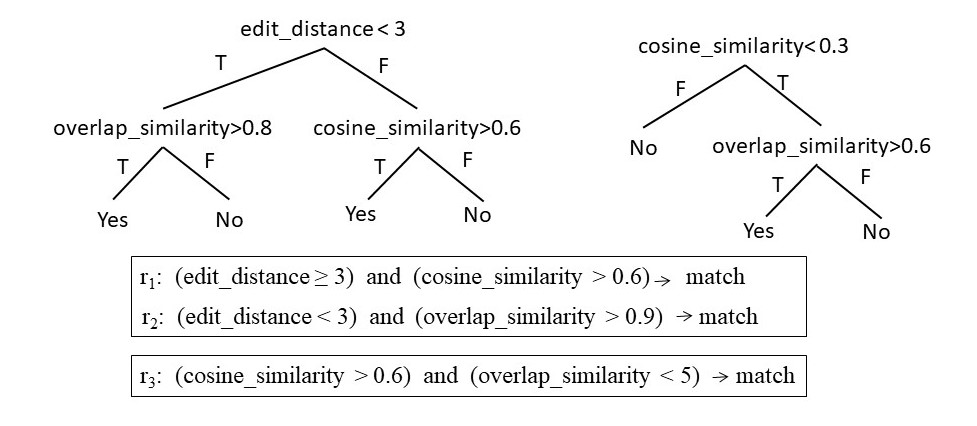
We show below a snippet of a random forest for blocking. A random
forest can also be viewed as a set of set of rules. The random
forest shown below is a set of two sets of rules. The arguments of
each predicate are two values to be compared.
Several general principles exist for automatically choosing the
similarity functions for blocking rules. For example, for a numerical
valued attributes such as age, weight, price, etc., candidate
similarity functions are: exact match, absolute difference, relative
difference, and Levenstein distance. For string valued attributes, it
is common to use edit distance, cosine similarity, Jaccard similarity,
and TF/IDF functions.
3.4 Active Learning of Random Forests
We can learn the random forest for the blocking rules through
the following active learning process. We randomly select a set of
pairs from the two datasets. By applying the similarity functions
on each pair, we obtain a set of feautres for each pair. Using
these features, we learn a random forest. We apply the resulting
rules to new pairs selected from the data set, and evaluate their
performance. If the performance is below a certain threshold, we
repeat the cycle, by providing additional labeled examples until an
acceptable performance is obtained. We illustrate this process
using the following example.
We assume that our first dataset contains three items: a, b, and c,
and our second dataset contains two items, d and e. From this dataset,
we pick two pairs (a,d) and (c,d) which are labeled by the user as
similar and not similar respectively. On this pair, we apply the
similarity functions each of which results in a feature of the
pair. We then use those features to learn a random forest. We apply
the learned rules to the tuples which were not in the training set,
and ask the user to verify the result. The user informs us that the
result for the pair (b,d) is incorrect. We add (b,d) to our training
set, and we repeat the process for another iteration. Over several
iterations, we anticipate the process to converge, and give us a
random forest that we can effectively use in the blocking step.
Once a radom forest has been learned, we present each of the learned rules to
the user. Based on the user verification, we choose the rules that will be
used in the subsequent steps.
3.5 Applying the Rules
Once we have learned the rules, the next step is to apply them on
the actual data. When the data size is huge, it is still not
possible to apply the blocking rules to all the pairs of objects.
Therefore, we resort to indexing. Suppose, one of the rules
requires that the Jaccard index should be greater than
0.7, and we are looking to match the movie Sound of
Music. As the length of the movie name is 3, we need consider only those
movies in our data whose length is between 3*0.7 and 3/0.7, ie,
between 2 and 4. If we have indexed the dataset on the size of the
movies, it is efficient to choose only those movies whose sizes are
between 2 and 4, and filter the set even further through the
application of the blocking rule.
3.6 Performing the Matching
The blocking step produces a much reduced set of pairs which must
be tested for whether they match. The general structure of the
matching process is very similar in that we first define a set of
features, learn a random forest, and through the active learning
process refine it. The primary difference between the blocking and the
matching step is that the matching process needs to be more exact and
can require more computation. That is because this is the final step
in the record linkage, and we need to have high confidence that the
two entities indeed match.
4. Summary
In this chapter, we considered the problem of creating a knowledge
graph by integrating the data coming from structured sources. The
integrated schema of the knowledge graph can be refined and evolved as
per the business requirements. The mappings between the schemas of
different sources can be bootstrapped through automated techniques,
but they do require verification through human input. Record
linkage is the integration of the data at the instance level where we
must infer the equality between two instances in the absence of
unique identifiers. The general approach for record linkage is to
learn a random forest through active learning process. For
applications requiring a high accuracy, automatically computed record
linkage may eventually need to undergo human verification.
Exercises
Exercise 4.1.Two
popular methods to calculate similarity between two strings are
edit distance (also known as Levenshtein distance) and the Jaccard measure.
We can define the
Levenshtein distance between two strings a, b (of length |a| and |b|
respectively), given by lev(a,b) as follows:
- lev(a,b) = a if |b| = 0
- lev(a,b) = b if |a| = 0
- lev(tail(a),tail(b)), if a[0] = b[0]
- 1 + min{lev(tail(a),b), lev(a,tail(b)), lev(tail(a),tail(b))} otherwise.
where the tail of some string x is a string of all but the first
character of x, and x[n] is the nth character of the string x,
starting with character 0.
We can define the Jaccard measure between two strings a, b
as the size of the intersection divided by the size of the
union between the two.
J(a,b) = |a ∩ b| / |a ∪ b|
|
(a) |
Given the strings "JP Morgan Chase" and "JPMC Corporation", what is the edit distance between the two? |
|
(b) |
Given the strings "JP Morgan Chase" and "JPMC Corporation", what is the Jaccard measure between the two? |
|
(c) |
Given three strings: x = Apple Corporation, CA, y = IBM Corporation, CA, and z =
Apple Corp, which of these strings would be equated by the edit distance methods? |
|
(d) |
Given three strings: x = Apple Corporation, CA, y = IBM Corporation, CA, and z =
Apple Corp, which of these strings will be equated by the Jaccard measure? |
|
(e) |
Given three strings: x = Apple Corporation, CA, y = IBM Corporation, CA, and z =
Apple Corp, what intuition you would use to ensure that x is equated to z? |
Exercise
4.2. A commonly used approach to account for the importance
of words is a measure known as TF/IDF. Term frequency (TF) denotes
the number of times a term occurs in a document. Inverse Document
Frequency (IDF) denotes the number of documents containing a term.
The TF/IDF score is calculated by taking the product of TF and
IDF. Use your intuition to answer whether the following is true
or false.
|
(a) |
Higher the TF/IDF score of a word, the rarer it is. |
|
(b) |
In a general news corpus, TF/IDF for the word Apple is likely to be higher than the TF/IDF for the word Corporation |
|
(c) |
Common words such as stop words will have a high TF/IDF. |
|
(d) |
If a document contains words with high TF/IDF, it is likely to be ranked higher by the search engines. |
|
(e) |
The concept of TF/IDF is not limited to words, and can also be applied to sequence of characters, for example, bigrams. |
Exercise
4.3. To check if two names might refer to the same
real-world organization, one strategy is to check the similarity
between two documents that describe them. Cosine similarity is a
measure of similarity between two vectors, and is defined as the
cosine of the angle between them. Highly similar documents will
have a cosine score closer to 1. Which of the following might be
a viable approach to convert a document into a vector for calculating
cosine similarity?
|
(a) |
Word embeddings of the words used in a document. |
|
(b) |
TF/IDF scores of the words used in a document. |
|
(c) |
TF/IDF of bigrams used in a document. |
|
(d) |
None of the above. |
|
(e) |
Any of (a), (b) or (c). |
Exercise
4.4. Which of the following is true about schema mappings?
|
(a) |
Schema mapping is largely an automated process. |
|
(b) |
It is usually straightforward to learn simple schema mappings. |
|
(c) |
Complete schema documentation is almost never available. |
|
(d) |
Examining the actual data in the two sources can provide important clues for schema mapping. |
|
(e) |
Database constraints play no role in schema mapping. |
Exercise
4.5. Which of the following is true about record linkage?
|
(a) |
Blocking can be an unnecessary and expensive step in the record linkage pipeline. |
|
(b) |
A random forest is a set of set of rules. |
|
(c) |
Blocking rules must always be authored manually. |
|
(d) |
Active learning of blocking rules minimizes the training data we must provide. |
|
(e) |
Matching rules are as expensive to apply as the blocking rules. |
|
 CS520
CS520