Section 2 - The Algorithms

2.1.1  Forward BWT

The BWT is applied on a 1-dimensional set of data. The output is generated according to the following scheme:

• All different rotations of the original data sequence are formed and arranged in a square matrix in ascending order whereby the elements of the first column are the most significant.
• Store the number of the row which contains the original sequence as the index I in order to allow the inverse transform to be successfully applied to the transformed sequence.
• Take the last column as the output of the transform.

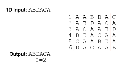
Fig. 1 Example of Burrows-Wheeler Transform

Figure 1 gives an example of the scheme.

2.1.2  Inverse Transform

Given the transformed vector L ( i.e. the last column in the matrix of Figure 1), and the index I, we can restore the original sequence S.

We observe the following

• The output vector of the BWT contains exactly the same number of occurrences of each symbol as the original sequence S. Therefore, sorting L yields the first column of the transformation pattern as illustrated in Figure 1.
• Furthermore, all sequences starting with the same symbol are sorted according to their second symbol.

As the first column contains the symbols that precede those in the last column (imagine the pattern to be spread over the surface of a cylinder rather than a plane) and as the first column is sorted anyway those rows whose last elements are equal are (among themselves) sorted with respect to the first column. In other words, those rows which have, for instance, symbol A as their last element in common are sorted in the same order as the rows which have A as their first element in common.

We create a one-to-one mapping table that maps the row number with the k^th occurrence of symbol A as the last element to the row number with the k^th occurrence of A in the first column.

The last element of S is simply the element of L at the position of the index.

Since the elements of the first column precede those in the last column as described above, we can now recursively reconstruct S from back to front obeying the following algorithm:

• Locate the current symbol in the last column and pick the element e of the first column but in the same row.
• Use mapping table to find the symbol in the last column that corresponds to the element e of the first column – the two symbols are equal due to the definition of the mapping table.
• e is now the current symbol.

Sorting algorithms are known to be among the most demanding of tasks in terms of computational complexity. Since we are applying the BWT to images containing a large amount of data, a straight-forward implementation will not show a satisfying performance. Our implementation consists of a radix-sort algorithm to pre-sort the data followed by a modified quicksort algorithm applied to the unsorted parts.

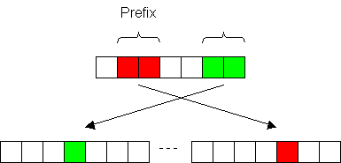
Fig. 2

Radix-Sort evaluates the prefix of each of the rotated sequences and distributes the sequences into N² bins where N is the magnitude of the alphabet. With simple arithmetic, the bin number can be directly determined as S1.N + S2, with S1 being the first of the two symbols and S2 the second. The advantage of this method clearly is that we do not have to occupy memory space for all of the possible rotations as we proceed along the initial vector picking one pair after the other. Note that subsequent pairs overlap, i.e. the second pair comprises the entries 2 and 3 as illustrated in figure 2.

As the prefixes are already sorted up to the depth of 2 (meaning the rotations are sorted with respect to the first two symbols), the following sorting can be applied to sets of rotations that match in their first two symbols.

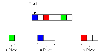
Fig. 3

Quicksort chooses one arbitrary (in our case, the first) element of the input vector as the so-called Pivot element. All other elements are compared to the Pivot and distributed into three bins depending on whether they are larger, equal or smaller in magnitude than the Pivot. The Pivot itself is put into the second bin as well. The three resulting sub-vectors are sorted by recursively applying the quicksort algorithm on each of them.

The standard quicksort algorithm had to be modified so that not only single elements are sorted but rather entire sequences. This is achieved by introducing the parameter depth which specifies the length of the prefixes that have already been sorted. The quicksort algorithm skips those elements that are already sorted and proceeds at the given depth. Furthermore, if all elements in a resulting sub-vector are equal at a certain depth the quicksort function is applied at depth+1.

2.2 Move-To-Front

The Move-To-Front (MTF) algorithm was part of the data compression algorithm defined in the original paper by Burrows and Wheeler. An MTF encoder keeps all possible data values in a list. It processes the input one value at a time by simply outputting that value's position in the list. It then moves this value to the top of the list. So, if the next value to be encoded is identical, this time it outputs a 0. On repetitive data, such as that produced by the BWT, an MTF encoder produces an output heavily weighted towards low integers and likely to include runs of those integers. These runs can then be run-length encoded.