Experiments

Design

There are several commonly used methods for quantifying subjective image quality.

a) Direct methods: subjects quantify their subjective impression of quality directly. This data are averaged between subjects. The main drawback is that this metric is unit-less, so it is hard to compare value across experiments.

b) Threshold judgments: These are based on the assumption that image fidelity is the same as image quality, which may not be true.

c) Pair-wise comparisons: Two images are compared to each other by several subjects. The percentage that one sample is preferred over the other is used as index of quality. This method provides very reliable data but requires too many comparisons.

The experiment method that I propose here aims to get the benefit of pair-wise comparisons but with much less comparisons:

a) For each original image, 18 JPEG images compressed at quality level from 5 to 39 with a step of 2.

b) These 18 JPEG images are blurred with a 3*3 filter to produce 18 blurred images.

c) Or these 18 JPEG images are post-processed using Chou et al’s de-blocking algorithm (1998).

So I will have totally 18*3=54 test images. Subjects are asked to rank these images by taking the worst image way (click it). In traditional ranking experiments, subjects have to do many pair comparisons for each images. But in this image set, we can safely assume that image quality is partially ranked already (inside each of the three categories). Thus we can arrange comparisons in a very efficient way. We always show subject three images (one from each category) at any time, subject is asked to choose the image with worst quality. This image is then taken away and the nearest image from the same category will replace it. Thus, subject only needs to do 53 comparisons, much less than a fully random ranking experiment. Before each comparison, image positions are randomly shuffled to avoid fix pattern effect. Below shows the interface of experiments.

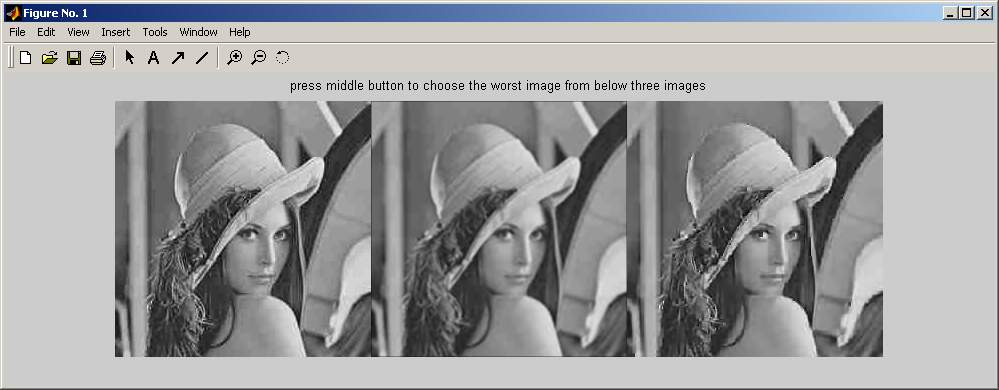
Figure 3. Subjective Testing Interface

Procedure

Two subjects, author and a friend of author took part in the experiments. Two 256 by 256 gray images, Lena & Einstein, are used. Each image is repeated 4 sessions and each session has 54 stimulus images. Images are displayed on the LCD screen of a HP OmniBook4150. View distance is approximately 16 inches. Ambient lighting is normal office condition.

Results and Analysis:

For each original image (Lena for example), we have totally 54 *4 (repeat)*2 (subjects) ranks. Average across repeat and subjects will give each stimulus image a score. This score is referred as the index of subjective quality. Figure 4-7 shows the comparison of different quality metrics with subjective quality. Good metrics should be monotonic. Although it is quite intuitive to see that the “mixed” metrics has the best shape (Fig 7) because the three curves for different categories almost overlap, we still need to compute a solid number. The method that I use here is:

Suppose the order of subjective quality for each stimulus is SO(i), the order of objective quality for each stimulus is OO(i). Then mean(|SO(i)-OO(i)|) will indicate how well the objective metrics correlates with subjective quality. Figure 8 is consistent with our intuition; the mean order error is the least for “mixed” metrics. A little bit surprising is that RMSE performances better than the more complicated BMR and EOBD metrics. I guess the reason is that pixel-based method is more reliable than other structure-based algorithm.

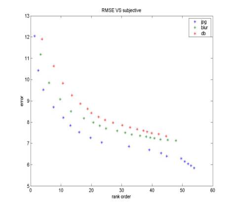
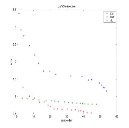
Figure 4. RMSE vs. Subjective Figure 5. BMR vs. Subjective

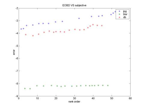
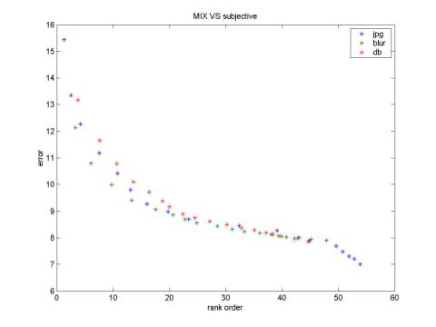
Figure 6. EOBD vs. subjective Figure 7. Mix vs. subjective

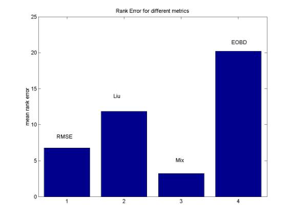
Figure 8. Rank Error for different image quality metrics