

The organization of the paper is as follows. First, we introduce some results from literature which pertain to our subject. Then, we present some observations regarding the general nature of audio signals. We then present theoretical descriptions of two algorithms, one which uses linear estimation and another which uses Principal Component Analysis components to hopefully capture the structure of a music signal. Finally, we present experimental results and our conclusion.
These approaches to wideband speech extrapolation all used non-linear models based upon the audible characteristics of the vocal tract. Each algorithm estimated frequency coefficients that were roughly between 4-8 kHz.
For the problem of wideband speech extrapolation, it has been reported that satisfactorily recovering the high frequency components of speech is impossible without side information ([7]). It is unclear whether this assertion would apply to other audio signals. A recent proposal by France Telecom, on bandwidth extrapolation for MPEG2001, is one of the first attempts to address the issue of extrapolating general audio signals. However, it requires the existence of additional side information pertaining to the high frequency characteristics of the signal.
Due to the predominance of quasi-stationary signal content in audio, the modified discrete cosine transform (MDCT) seemed a natural transform to apply before analyzing each audio signal. This is because the MDCT eliminated spurious tones created by blocking artifacts without increasing the number of parameters which we would need to analyze.
As an aside, it was found that with the high frequencies, error concealment could effectively mask the loss of any high frequency components. By error concealment, what is meant is the common practice of using old frequency components from a previous block or frame in lieu of any currently missing frequency components. Keeping every other high frequency and zeroing out the rest, however, resulted in audible distortions. Repeated low frequencies also created more irritating audible distortions.
Sample1 original | Sample1
of error concealment data | Sample1
of every other high frequency block zeroed
Sample2 original | Sample2
of error concealment data | Sample2
of every other high frequency block zeroed
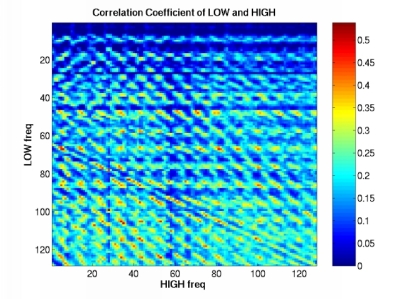
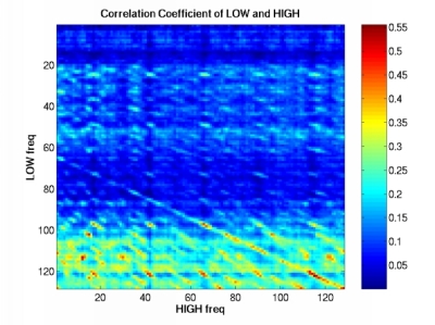
After applying the MDCT, the frequencies were separated into high and
low subsets, and the correlation coefficients were calculated for each
audio signal.
|
|
|
|
|
|
|
|
|
|
|
|
As shown by the plots, the correlation between high and low frequencies varied widely amongst the different audio signals. In particular, the high frequency coefficients in the voice and mixed audio signals were largely uncorrelated, which they exhibited periodic correlations in the cello signal.
There are also several interesting general observations to be made. First of all, the high frequency components comprise only a small fraction of the total energy of the signal. These components nonetheless add a perceptually audible quality to their signal. The distribution of values for each frequency bin exhibited Laplacian distribution for all the frequency bins and for all the data that we encountered.
Our exploratory studies also revealed that randomly distorting the phase of the high frequency coefficients did not create any audible distortion. High frequency can be loosely defined as the frequency range above 5.5kHz in our audio samples. For cello sample, that range can be as low as 4kHz due to lack of energy concentration in the high frequency region. Since the MDCT is a real valued transform, such phase adjustments would be equivalent to randomly multiplying the coefficients by 1 or -1. However, as with the case for error concealment, distorting the lower frequencies in such a manner created audible distortion.
Sample1 original | Sample1
of random phase of high frequency | Residue
between sample1 and original
Sample2 original | Sample2
of random phase of high frequency | Residue
between sample2 and original
 |
|
|
The algorithms, while different, share several general characteristics. Each approach requires that we divide the spectrum into low frequencies which are available as input, and high frequencies which are unavailable and need to be estimated. As this distinction would be rather application-specific, we varied the cutoff frequency between the two subsets throughout or experiments. Furthermore, since random high frequency phase distortion of audio signals did not degrade their perceptual quality, it was deemed appropriate to simplify the problem by only estimating the envelope of the high frequency spectrum. Afterwards, the sign of each component could be randomly adjusted to produce a signal with random phase distortion. Finally, each approach is similar in that it required a training session with wideband data. The dissimilarities of each approach are discussed below.
Training consists of minimizing the squared error on the training data set. However, this often leads to overfitting. In order to reduce overfit, low-order linear estimators were explored, where each high frequency coefficient estimate was a linear function of a sparse number of low frequency coefficients. The low frequency coefficients could either be chosen according to their relative magnitude or their cross correlation with each particular high frequency coefficient.
In mathematical terms, given MDCT envelope coefficients ![]() from the training data, let X be defined as follows:
from the training data, let X be defined as follows:
Given cutoff frequency f which divides the frequency bins into
low and high components, define ![]() and
and ![]() such that
such that
![]()
The the weights w which give the least-squares fit to the training data are given by:
![]()
The low order estimator is given by presetting some of the weights to zero, and then fitting the remaining weights to minimize the mean squared error. As stated previously, the weights which correspond to the frequency bins with the largest correlation coefficient are the ones which should be chosen. Alternately, one might also simplify the algorithm by choosing the weights which correspond to the frequency bins with the largest power, but this naturally does not work as well.
Given ![]() ,
, ![]() , and
, and ![]() defined as before, let
defined as before, let ![]() be the autocorrelation matrix of the envelope of low frequency components
of the training data. Then there exists diagonal matrix
be the autocorrelation matrix of the envelope of low frequency components
of the training data. Then there exists diagonal matrix ![]() , whose diagonal elements
, whose diagonal elements ![]() are in order of decreasing absolute value, and orthonormal matrix
are in order of decreasing absolute value, and orthonormal matrix ![]() such that
such that ![]() . This is the SVD decomposition for
. This is the SVD decomposition for ![]() . Enumerate the columns of
. Enumerate the columns of ![]() as
as ![]() . For n<N, let
. For n<N, let ![]() be defined as follows:
be defined as follows:
We seek to find a matrix of weights ![]() which satisfy the following property:
which satisfy the following property:
![]()
This approach is similar to the normal low-order linear least squares estimator; however, each high frequency estimate is a weighted combination of all the low frequency components projected onto various principal component directions. By reducing the order of the estimator in this manner, we hope to reduce the possibility of overfit while still preserving the ability to estimate realistic audio signals.
For the linear estimate, we varied the cutoff frequency that separates the low frequency input features from the high frequency desired output. Naturally, the estimated signal was degraded as the cutoff frequency was lowered. We also varied the number of weights of the linear estimator, trying to reduce its tendency towards overfit without compromising its ability to fit the training data.
For the PCA estimator, we deemed it unnecessary to vary the cutoff frequency and focused on finding the optimal number of basis vectors to include. This is analogous to varying the number of weights in the linear estimator since in both cases we are reducing the order of the estimator to reduce overfit.
The results of each experiment was evaluated according to its squared error distortion (or signal to noise ratio), and by its perceptual quality. In most cases the two criteria were in agreement although this was not always the case.
Overall, training either estimator on a portion of a song and testing it on another portion from that same song generally gave good results. However, neither algorithm gave satisfactory results when the test and training data were from different songs, even when the songs seemed perceptually similar. We now proceed to give our detailed results and our explanations in the section below.
First of all, the correlation between frequency bins varied widely from song to song, even between two songs performed by the same musician on the same instrument. As a result, training the weights on one song produced severe squared error terms in another song. Second of all, even when the squared error was small, it did not guarantee any perceptual improvement in the quality of sounds. This is partly because the high frequency coefficients are very small and insignificant from a mean squared sense even though they definitely have a perceptible impact on the signal sound.
In other words, linear weights did a poor job of reducing the squared error, and in any case reducing the squared error did not necessarily result in improved perceptual quality. The detailed results are as follows.
First, we partitioned a single music file - a song performed on the
cello - into training and test data. We chose the weights by taking a linear
least squares fit between the low and high frequency envelopes, with resulting
training and test error. We repeated these tests, dividing the low and
high frequency ranges between a range of cutoff frequencies. The resulting
squared error as a function of cutoff frequency is as plotted below:
 |
This squared error was roughly a 50% improvement over the error which
would result without any linear estimation at all, which is plotted below:
 |
As seen from the plot, increasing the cutoff frequency (thereby reducing the number of high frequency coefficients to be estimated) reduced the resulting squared error. Furthermore, the weights predicted the training and test sequences almost equally well, denoting a relative lack of overfit. This would suggest that weights trained on a portion of a song would predict well for the song's duration.
Perceptually the test results matched the squared error analysis, in the the test data sounded only slightly worse than the training data. Included are two .wav files, which show how the linear estimation changed the perceptual quality of the sound. The bandwidth extrapolation seemed to have the effect of adding qualities of the original instrument and high frequency noise, as can be heard from the links below:
Sample of original wideband test data | Same sample, but bandlimited | Same sample after bandwidth extrapolation
However, applying the weights to a different song - still performed
on the cello by the same musician - produced poor results. For all choices
of cutoff frequency, the weights suffered from severe overfitting, as shown
in the plot below:
 |
As shown by the figure, the weights generalized very poorly to a different song, even though the song perceptually shared similar characteristics to the training data. From a perceptual standpoint the tests again produced poor results, as shown by the .wav files included below. This overfit can be clearly heard in the form of noise in the estimated data files, linked below:
Original wideband test file | Bandlimited test data, before estimation | After estimation
In order to mitigate the overfitting, we trained a reduced order linear
estimator. This time, we limited the number of weights involved. Again,
we trained the weights on one song and tested the weights on another separate
though perceptually similar song. Setting the cuttof frequency to 4.1 kHz
and varying the order of the estimator produced the following SNR plot:
 |
As shown by the plot, a low order estimator is relatively effective in controlling overfit, at least in comparison to the test results with a dense weight set. However, perceptually the low order estimator still produced very poor results. In order to avoid overfitting, the low order estimator makes extremely conservative estimates which turn out to be audibly imperceptible. These perceptual results are in accordance with the poor signal to noise ratio of the estimated signal.
Original wideband file | Bandlimited data before estimation | After estimation
Our implementation of PCA compacted most of the narrowband signal energy
into a reduced number of basis functions. In the figure below, we show
the energy concentration as a function of the number of components incorporated
in the approximation process. Note that the close to 95 percent of the
signal energy is concentrated in the 20 most principal component vectors.
The SNR of low frequency and approximated low frequency using different
number of eigenvectors is shown in the figure. The two curves represent
PCA applied to the envelope of the low frequency and the signed low frequency.
Here it suggests again that dealing with only the envelopes is a simpler
and more effective method.
 |
|
|
We then generated a set of linear weights to estimate the high frequency coefficients from the principal component vectors. The linear estimation is applied to the reduced order of PCA coefficients and the high frequency envelope of the training data. For an unbiased estimator both the PCA coefficients and the high frequency has to be centered to it mean. This subtraction of the mean in both domain results in discrepancy in the cross validation step.
After the training, the low frequency envelope of the test data is decomposed into principal component parameters and used in the estimation of the high frequency envelope. The same estimation process as in the training data is applied to the test data with assumption that the statistical characteristics of the training data and the test data are almost identical. The unbiased estimator estimates the deviation from the mean of the high frequency envelope of the training data.
The following figure illustrates the SNR of the estimation process.
Linear estimation trained on the training data and tested on a subset of
the training data is first shown. The best SNR is naturally achieved by
incorporating all the eigenvectors. Unfortunately, the best SNR is not
much greater than 4 dB, indicating that there is very little correlation
between the low frequency envelope and the high frequency envelope. Two
other plots show the cross validation of the estimation process. For the
cello case, incorporating more than 60 components does not improve the
SNR of the estimation done on test data. Two different mean values were
added to the unbiased estimation of the high frequency envelope. First,
the mean of the high frequency envelope of the training data (unknown HIGH
mean) was added under the assumption that the statistical characteristics
of the test and training data are same. Second, the mean value of the test
data high frequency envelope (known HIGH mean) was added to the unbiased
estimated envelope for comparison. The assumption of almost identical statistical
characteristics between the training and test data set does not hold in
general as can be seen by the discrepancy in the figure. Same figure of
SNR and the order of the PCA coefficients for a different audio sample
(vega), i.e. voice music piece, is also given for comparison.
 |
 |
Although the SNR (or MSE) and the perceptual quality does not always
correspond, the 'best' SNR giving parameters were used to reconstruct estimated
wideband audio signals for cello and vega. The cello sequence exhibits
a slight improvement in the sharpness, although there are still artifacts.
For the vega sequence, improvement in the sharpness is accompanied by noisy
distortions. In both the sequences, such noise artifacts to be much more
audible when the there is an increase in the audio signal itself. Such
phenomena was audible in other reconstructed audio samples not provided
and they suggest further investigation.
| Narrowband signal | Reconstructed signal | Original signal | |
| Cello sample | Cello Narrowband | Cello Reconstructed | Cello Original |
| Vega sample | Vega Narrowband | Vega Reconstructed | Vega Original |
As a continuation of the sparse selective linear estimation, low frequency
for the vega sample was redefined as the upper region of the low frequency
since there was correlation only in that region. Figure shows the SNR and
the order of the parameterization. Although smaller order of coefficients
was realizable for the same SNR as the experiment prior, there was no gain
in the perceptual quality.
 |
Vega sample reconstructed with only the region of the low frequency
The most serious weakness of this approach is that the majority of audio signals that we tested had frequency coefficients that were largely uncorrelated. This right away ruled out frequency-domain based linear estimation for most audio signals. Our usage of the MDCT was motivated by the fact that transform methods are commonly used in compression to eliminate redundancy and reduce the description length of sinusoidal data. However, for the signals which we tested the MDCT produced coefficients which were uncorrelated and therefore difficult to predict.
PCA captured the energy concentration characteristics of the signal, but it failed in effective reduction of dimensionality in describing the low frequency. As can be seen from the small correlations between frequency bins, energy distribution in the frequency does not correspond to an effective description of the low frequency. Also, PCA exploits only up to second order statistics of the given signal. Therefore, a Gaussian distributed signal is completely described by PCA, but the distribution of frequency coefficients of all our samples exhibit Laplacian distribution. Therefore, a different method of component analysis, such as the Independent Component Analysis, may be more effective in describing the low frequency in lower order.
Although there are extensions to the estimation process, such as nonlinear methods, we feel that it is important that the low frequency be accurately described in a lower dimension. This would give a better understanding of the signal in frequency domain and will facilitate the estimation process, whatever that may be.
A direction for future research would be to preprocess
the data using some alternative to linear transform methods. For example,
one way to efficiently capture the structure of music would be to employ
models based on the audible physics of musical instruments. For example,
a rather peculiar model developed in 1877 is the 1 dimensional
mechanical analog of a stringed instrument played by a bow:
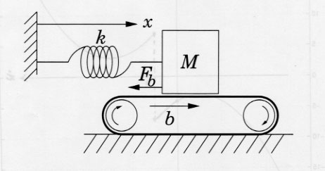
Using an accurate model would reduce the complexity of describing music to specifying the spring/mass constants, and the speed of the conveyor belt. If parameters such as these could be estimated from bandlimited data then bandwidth extrapolation would be possible.
We found work done on a variety of parametric models
that are tailored for representing audio signals in the late stage of our
project. Although, we could not delve deep into it for this project,
it is a material that catch our attention for further investigation to
the problem.
2. M. Bosi, "EE 367C course reader." [perceptual audio coding]
3. Y.M. Cheng, D. O'Shaugnessy & P. Mermelstein, "Statistical recovery of wideband speech from narrowband speech," IEEE Trans. Speech Audio Process., vol. 2, pp. 544-548, 1994.
4. J. Epps & W.H. Holmes, "A new technique for wideband enhancement of coded narrowband speech," Proc. IEEE Speech Coding Workshop (Porvoo Finland), 1999, pp. 174-176.
5. S. Gustafsson, P. Jax & P. Vary, "A Novel Psychoacoustically Motivated Audio Enhancement Algorithm Preserving Background Noise Characteristics," Proceedings of the IEEE International Conference on Acoustics, Speech, and Signal Processing, Vol. 1, pp. 397-400, 1998.
6. T. Painter & A. Spanias, "Perceptual coding of digital audio.", Proceeding of the IEEE, April 2000.
7. J. Valin & R. Lefebvre, "Bandwidth extension of narrowband speech for low bit-rate wideband coding.", IEEE Speech Coding Workshop, 17-20 Sep. 2000, pp. 130-132.
8. Lord Rayleigh, "The Theory of Sound", 1877
9. Micahel M. Goodwin, "Adaptive Signal Models : Theory, Algorithms, and Audio Applications", Ph. D. dissertation, Memorandum no. UCB/ERL M97/91, Electronics Research Laboratory, College of Engineering, University of California, Berkeley, 1997