Least-Squares Line

Stats 203

Stanford University

Estimating the Age of the Universe

Comparing Lines of Best Fit

All of us got different lines. How do we know which line is best?

Calculate the sum of squared errors between the points and the line.

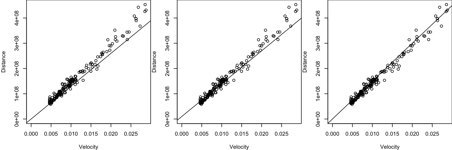
Comparing Lines of Best Fit

All of us got different lines. How do we know which line is best?

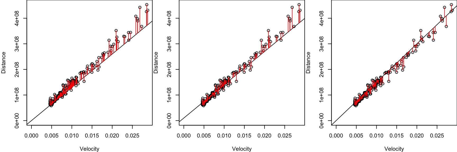
Calculate the sum of squared errors between the points and the line.

\[\text{SSE}(\alpha, \beta) = \sum_{i=1}^n (y_i - (\alpha + \beta x_i))^2\]

Sum of Squared Errors

\[\text{SSE}(\alpha, \beta) = \sum_{i=1}^n (y_i - (\alpha + \beta x_i))^2\]

How do we find the values of \(\alpha\) and \(\beta\) that minimize \(\text{SSE}\)?

Least-Squares Line

To minimize \(\text{SSE}(\alpha, \beta) = \sum_{i=1}^n (y_i - (\alpha + \beta x_i))^2\), take derivatives, set equal to \(0\), and solve for \((\alpha, \beta)\).

\[ \frac{\partial (\text{SSE})}{\partial \alpha} = 0 \]

\[ \frac{\partial (\text{SSE})}{\partial \beta} = 0 \]

\[ \hat{\alpha} = \bar y - \hat{\beta} \bar x \]

\[ \hat\beta = \frac{\sum_{i=1}^n (x_i - \bar x)(y_i - \bar y)}{\sum_{i=1}^n (x_i - \bar x)^2} \]

Calculating the Least-Squares Line

\[ \begin{align*} \hat{\alpha} &= \bar y - \hat{\beta} \bar x & \hat\beta &= \frac{\sum_{i=1}^n (x_i - \bar x)(y_i - \bar y)}{\sum_{i=1}^n (x_i - \bar x)^2} \end{align*} \]

The lm function in R calculates these coefficients for you.

Predicting with Least-Squares

The least-squares line is \[ \hat y = -3931447 + 14853755377 x. \]

How far is a supernova that is moving away at a velocity of \(0.020\) parsecs/year?

Simply plug \(x = 0.020\) into the equation of the line: \[ \hat y = -3931447 + 14853755377 (0.020) = 293143661 \text{ (parsecs)}. \]

R can make predictions for you, but the data must be in a data.frame.

Interpreting the Least-Squares Line

Least-Squares Line

The least-squares line, also called the regression line, is \(\hat y = \hat\alpha + \hat\beta x\), where \[ \begin{align*} \hat{\alpha} &= \bar y - \hat{\beta} \bar x & \hat\beta &= \frac{\sum_{i=1}^n (x_i - \bar x)(y_i - \bar y)}{\sum_{i=1}^n (x_i - \bar x)^2}. \end{align*} \]

How do we interpret this line?

• By rearranging the expression for \(\hat\alpha\), we see that the line passes through \((\bar x, \bar y)\): \[ \bar y = \hat\alpha + \hat\beta \bar x. \] In other words, the predicted value for \(\bar x\) is \(\bar y\).
• The slope can also be expressed as \[ \hat\beta = r \frac{s_y}{s_x}. \]

Interpreting the Least-Squares Line

To understand this formula, let’s look at Galton’s study of heights of parents and offspring, which led him to coin the term “regression”.

Galton’s Heights

What is the relationship between heights of fathers and their children?

Heights of Fathers and Sons

\[\hat\beta = r\frac{s_y}{s_x} \approx 0.4\]

What would you predict is…

• the height of a son whose father is 70.2 in. tall (1 in. above average)?
• the height of a son whose father is 67.2 in. tall (2 in. below average)?

Francis Galton called this phenomenon regression to the mean, which is why the least-squares line is often called the regression line.

Visualizing the Regression Line

A Regression Paradox

Earlier, we saw that a 70.2 in. tall father (1 in. above average) is predicted to have a son who is 69.6 in. tall (0.4 in. above average).

Now, if a son is 69.6 in. tall, what is the predicted height of the father?

Moral: The regression of \(Y\) on \(X\) is not the same as the regression of \(X\) on \(Y\).

The Linear Algebra Perspective

Linear Algebra Connection

Suppose we have \(n\) observations: \((x_1, y_1), (x_2, y_2), \dots, (x_n, y_n)\).

We can write this in terms of vectors

\[ \begin{align} {\bf x} &= (x_1, x_2, \dots, x_n) & {\bf y} &= (y_1, y_2, \dots, y_n) \end{align} \]

The corresponding fitted values are: \[ \begin{pmatrix} \hat y_1 \\ \hat y_2 \\ \vdots \\ \hat y_n \end{pmatrix} = \begin{pmatrix} \alpha + \beta x_1 \\ \alpha + \beta x_2 \\ \vdots \\ \alpha + \beta x_n \end{pmatrix} = \alpha \begin{pmatrix} 1 \\ 1 \\ \vdots \\ 1 \end{pmatrix} + \beta \begin{pmatrix} x_1 \\ x_2 \\ \vdots \\ x_n \end{pmatrix}. \]

Linear Algebra Connection

Suppose we have \(n\) observations: \((x_1, y_1), (x_2, y_2), \dots, (x_n, y_n)\).

We can write this in terms of vectors

\[ \begin{align} {\bf x} &= (x_1, x_2, \dots, x_n) & {\bf y} &= (y_1, y_2, \dots, y_n) \end{align} \]

The corresponding fitted values are: \[ \underbrace{\begin{pmatrix} \hat y_1 \\ \hat y_2 \\ \vdots \\ \hat y_n \end{pmatrix}}_{\hat{\bf y}} = \begin{pmatrix} \alpha + \beta x_1 \\ \alpha + \beta x_2 \\ \vdots \\ \alpha + \beta x_n \end{pmatrix} = \alpha\, \underbrace{\begin{pmatrix} 1 \\ 1 \\ \vdots \\ 1 \end{pmatrix}}_{{\bf 1}} + \beta\, \underbrace{\begin{pmatrix} x_1 \\ x_2 \\ \vdots \\ x_n \end{pmatrix}}_{{\bf x}}. \]

The vector of fitted values \(\hat {\bf y}\) is a linear combination of \({\bf 1}\) and \({\bf x}\), so it is in their span: \[ \hat {\bf y} \in \text{span}({\bf 1}, {\bf x}). \]

Least-Squares Line and Projection

Remember that we choose \(\alpha\) and \(\beta\) to minimize

\[ \begin{align} \text{SSE}(\alpha, \beta) &= \sum_{i=1}^n (y_i - (\alpha + \beta x_i))^2 \end{align} \]

This is equivalent to choosing \(\hat{\bf y}\) to minimize

\[ \begin{align} || {\bf y} - &\hat{\bf y} ||^2 \\ \text{subject to } &\hat {\bf y} \in \text{span}({\bf 1}, {\bf x}) \end{align} \]

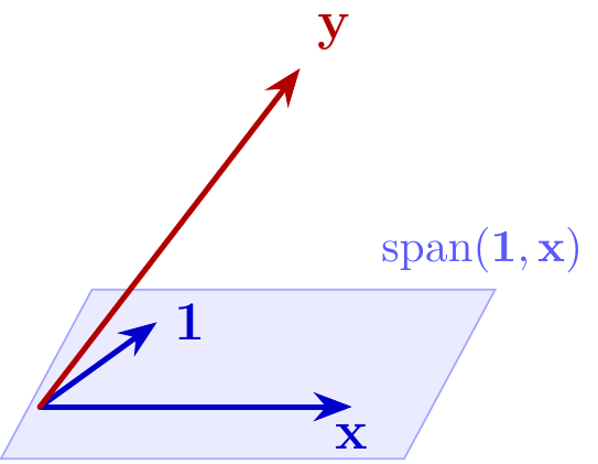
Visualization for \(n = 3\)

Least-Squares Line and Projection

Remember that we choose \(\alpha\) and \(\beta\) to minimize

\[ \begin{align} \text{SSE}(\alpha, \beta) &= \sum_{i=1}^n (y_i - (\alpha + \beta x_i))^2 \end{align} \]

This is equivalent to choosing \(\hat{\bf y}\) to minimize

\[ \begin{align} || {\bf y} - &\hat{\bf y} ||^2 \\ \text{subject to } &\hat {\bf y} \in \text{span}({\bf 1}, {\bf x}) \end{align} \]

which is \(P_{\text{span}({\bf 1}, {\bf x})}{\bf y}\), the projection of \({\bf y}\) onto the span.

Visualization for \(n = 3\)

Applications of Linear Algebra

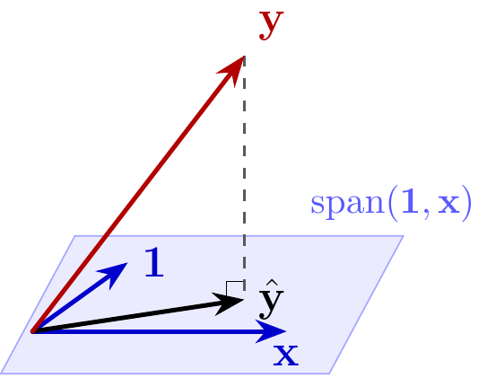
1. We see that \({\bf y} - \hat{\bf y}\) is orthogonal to both \({\bf 1}\) and \({\bf x}\), so

   • \(0 = {\bf 1} \cdot ({\bf y} - \hat{\bf y}) = \sum_{i=1}^n (y_i - (\alpha + \beta x_i))\)
   • \(0 = {\bf x} \cdot ({\bf y} - \hat{\bf y}) = \sum_{i=1}^n x_i (y_i - (\alpha + \beta x_i)),\)

   which are the equations that we solve for \(\alpha\) and \(\beta\) (no derivatives required)!

2. By the Pythagorean Theorem, we see that

   • \(||\hat{\bf y}||^2 + ||{\bf y} - \hat{\bf y}||^2 = ||{\bf y}||^2\)
   • or equivalently \[ \sum_{i=1}^n \hat y_i^2 + \sum_{i=1}^n (y_i - \hat y_i)^2 = \sum_{i=1}^n y_i^2. \]

   This identity is not easy to prove by algebra!

Recap

• The least-squares line minimizes \(\text{SSE}(\alpha, \beta) = \sum_{i=1}^n (y_i - (\alpha + \beta x_i))^2\), or equivalently \(|| {\bf y} - \hat{\bf y} ||^2\) subject to \(\hat{\bf y} \in \text{span}({\bf 1}, {\bf x})\).
• The slope is \(\hat{\beta} = r \frac{s_y}{s_x}\), and the line passes through \((\bar{x}, \bar{y})\).
  • Regression to the mean: Since \(|r| \le 1\), predictions will be closer to the mean.
• The predicted value of \(y\) can be obtained as \(\hat y = \hat\alpha + \hat\beta x\).

Next time: The linear regression model (with assumptions about distributions).