The Linear Regression Model
Stats 203
Stanford University
The Linear Regression Model
Linear Regression Model
The linear regression model assumes that the data are generated as \[ \begin{align} Y_i &= \alpha + \beta x_i + \epsilon_i, & i=1, 2, \dots, n \end{align} \]
where \(x_i\) are fixed and \(\epsilon_i \overset{i.i.d.}{\sim} \text{Normal}(0, \sigma^2)\).
Alternative descriptions:
- \(Y_i \sim \text{Normal}(\alpha + \beta x_i, \sigma^2)\), independent
- \(Y_i \mid X_i = x \sim \text{Normal}(\alpha + \beta x, \sigma^2)\), independent
Estimating Parameters
To estimate parameters in the linear regression model, we use maximum likelihood (as in any probabilistic model).
\[ {\small L(\alpha, \beta, \sigma^2) = \frac{1}{\sqrt{2\pi \sigma^2}} e^{-\frac{1}{2\sigma^2} (y_1 - (\alpha + \beta x_1))^2} \dots \frac{1}{\sqrt{2\pi \sigma^2}} e^{-\frac{1}{2\sigma^2} (y_n - (\alpha + \beta x_n))^2}} \]
We usually take logs.
\[ \ell(\alpha, \beta, \sigma^2) = -\frac{n}{2} \log(2\pi \sigma^2) - \frac{1}{2\sigma^2} \sum_{i=1}^n (y_i - (\alpha + \beta x_i))^2. \]
Estimating Coefficients
\[ \ell(\alpha, \beta, \sigma^2) = -\frac{n}{2} \log(2\pi \sigma^2) - \frac{1}{2\sigma^2} \sum_{i=1}^n (y_i - (\alpha + \beta x_i))^2. \]
To estimate \(\alpha\) and \(\beta\), we maximize \(\ell\)—which, as a function of \(\alpha\) and \(\beta\), is of the form \[ \text{constant} - \text{constant} \sum_{i=1}^n (y_i - (\alpha + \beta x_i))^2. \]
That is, to maximize the (log-)likelihood, it is equivalent to minimize \[ \sum_{i=1}^n (y_i - (\alpha + \beta x_i))^2. \]
But this is just the SSE criterion from last time!
In other words, the least-squares coefficients are also the MLE.
Estimating Error Variance
\[ \ell(\alpha, \beta, \sigma^2) = -\frac{n}{2} \log(2\pi \sigma^2) - \frac{1}{2\sigma^2} \sum_{i=1}^n (y_i - (\alpha + \beta x_i))^2. \]
To estimate \(\sigma^2\), we plug in the least-squares estimates \(\hat\alpha\) and \(\hat\beta\) (which do not depend on \(\sigma^2\)), and maximize \[ -\frac{n}{2}\log(2\pi) - \frac{n}{2}\log(\sigma^2) - \frac{1}{2\sigma^2} \sum_{i=1}^n (y_i - (\hat\alpha + \hat\beta x_i))^2. \]
Taking derivatives with respect to \(\sigma^2\), we obtain: \[ - \frac{n}{2\sigma^2} + \frac{1}{2(\sigma^2)^2} \sum_{i=1}^n (y_i - (\hat\alpha + \hat\beta x_i))^2 = 0, \]
and solving for \(\sigma^2\), we obtain \(\displaystyle \hat\sigma^2 = \frac{1}{n} \sum_{i=1}^n (y_i - (\hat\alpha + \hat\beta x_i))^2\).
Unbiased Estimator of Error Variance
The problem with \(\displaystyle \hat\sigma^2 = \frac{1}{n} \sum_{i=1}^n (y_i - (\hat\alpha + \hat\beta x_i))^2\) is that it is biased for \(\sigma^2\).
\[ E\left[ \hat\sigma^2 \right] = \frac{n-2}{n} \sigma^2 \]
We can obtain an unbiased estimator by dividing by \(n-2\) instead of \(n\): \[ S^2 = \frac{1}{n-2} \sum_{i=1}^n (y_i - (\hat\alpha + \hat\beta x_i))^2. \]
Consequences
Unbiasedness of \(\hat\beta\)
Recall that \(\hat\beta = \dfrac{\sum_{i=1}^n (x_i - \bar{x})(Y_i - \bar{Y})}{\sum_{i=1}^n (x_i - \bar{x})^2}\).
The easiest way to calculate the expectation is to first write \[ Y_i - \bar Y = (\alpha + \beta x_i + \epsilon_i) - \frac{1}{n} \sum_{j=1}^n (\alpha + \beta x_j + \epsilon_j) = \textcolor{red}{\beta (x_i - \bar x) + (\epsilon_i - \bar\epsilon)}, \]
and substitute into the expression above: \[ \hat\beta = \dfrac{\sum_{i=1}^n (x_i - \bar{x})\left[\textcolor{red}{\beta (x_i - \bar{x}) + (\epsilon_i - \bar \epsilon)}\right]}{\sum_{i=1}^n (x_i - \bar{x})^2} = \beta + \dfrac{\sum_{i=1}^n (x_i - \bar{x})(\epsilon_i - \bar{\epsilon})}{\sum_{i=1}^n (x_i - \bar{x})^2}. \]
Taking expectations (using \(E[\epsilon_i] = E[\bar\epsilon] = 0\)):
\[ E[\hat\beta] = \beta + \frac{\sum_{i=1}^n (x_i - \bar{x})\, E[\epsilon_i - \bar\epsilon]}{\sum_{i=1}^n (x_i - \bar{x})^2} = \beta. \qquad \checkmark \]
Variance of \(\hat\beta\)
The easiest way to calculate the variance is to use \(\sum (x_i - \bar x) = 0\) to write
\[ \hat\beta = \dfrac{\displaystyle\sum_{i=1}^n (x_i - \bar{x})(Y_i - \bar{Y})}{\displaystyle\sum_{i=1}^n (x_i - \bar{x})^2} = \dfrac{\displaystyle \sum_{i=1}^n (x_i - \bar{x})Y_i}{\displaystyle \sum_{i=1}^n (x_i - \bar{x})^2} - \underbrace{\dfrac{\displaystyle \sum_{i=1}^n (x_i - \bar{x})\bar Y}{\displaystyle \sum_{i=1}^n (x_i - \bar{x})^2}}_0. \]
Taking variances (recalling that \(\text{Var}[cW] = c^2 \text{Var}[W]\) and \(\text{Var}[V + W] = \text{Var}[V] + \text{Var}[W]\) when \(V\) and \(W\) are independent):
\[ \text{Var}[\hat\beta] = \dfrac{\displaystyle \sum_{i=1}^n (x_i - \bar x)^2 \text{Var}[Y_i]}{\displaystyle \left( \sum_{i=1}^n (x_i - \bar x)^2 \right)^2} \phantom{= \frac{\sigma^2}{\displaystyle\sum_{i=1}^n (x_i - \bar x)^2}.} \]
Variance of \(\hat\beta\)
The easiest way to calculate the variance is to use \(\sum (x_i - \bar x) = 0\) to write \[ \hat\beta = \dfrac{\displaystyle\sum_{i=1}^n (x_i - \bar{x})(Y_i - \bar{Y})}{\displaystyle\sum_{i=1}^n (x_i - \bar{x})^2} = \dfrac{\displaystyle \sum_{i=1}^n (x_i - \bar{x})Y_i}{\displaystyle \sum_{i=1}^n (x_i - \bar{x})^2} - \underbrace{\dfrac{\displaystyle \sum_{i=1}^n (x_i - \bar{x})\bar Y}{\displaystyle \sum_{i=1}^n (x_i - \bar{x})^2}}_0. \]
Taking variances (recalling that \(\text{Var}[cW] = c^2 \text{Var}[W]\) and \(\text{Var}[V + W] = \text{Var}[V] + \text{Var}[W]\) when \(V\) and \(W\) are independent):
\[ \text{Var}[\hat\beta] = \dfrac{\displaystyle \sum_{i=1}^n (x_i - \bar x)^2 \text{Var}[Y_i]}{\displaystyle \left( \sum_{i=1}^n (x_i - \bar x)^2 \right)^2} = \frac{\sigma^2}{\displaystyle\sum_{i=1}^n (x_i - \bar x)^2}. \]
Sampling Distribution of \(\hat\beta\)
From the previous slide, we see that \[ \hat\beta = \sum_{i=1}^n \underbrace{\frac{(x_i - \bar x)}{\sum_{j=1}^n (x_j - \bar x)^2}}_{c_i} Y_i, \]
a linear combination of the independent normal random variables \(Y_1, \dots, Y_n\).
Any linear combination of independent normals is also normal, so \[ \hat\beta \sim \text{Normal}\left(\beta, \frac{\sigma^2}{\sum_{i=1}^n (x_i - \bar x)^2}\right). \]
Simulating the Sampling Distribution
\[ \hat\beta \sim \text{Normal}\left(\beta, \frac{\sigma^2}{\sum_{i=1}^n (x_i - \bar x)^2}\right). \]
We can convince ourselves of this by simulation.
Assumptions and Diagnostics
The problem with a model is that everything depends on whether it is correct.
Assumptions
\[ \begin{align} Y_i &= \alpha + \beta x_i + \epsilon_i, & \epsilon_i &\sim \text{Normal}(0, \sigma^2) & i=1, \dots, n \end{align} \]
What are the assumptions in this expression?
- Linearity: The mean of \(Y\) is linear in \(x\).
- Homoskedasticity: \(\epsilon_i\) has constant variance.
- Normal errors: \(\epsilon_i\) is normal.
- Independence: \(\epsilon_i\)s are independent.
How do we know if these assumptions are satisfied?
Residuals
We do not observe the error \[ \epsilon_i = Y_i - (\alpha + \beta x_i), \]
but we can estimate it by the residual \[ e_i = Y_i - \underbrace{(\hat\alpha + \hat\beta x_i)}_{\hat Y_i}. \]
We can use the residuals to diagnose violations of the assumptions.
Residual Plot
A residual plot is a plot of the residuals versus \(x\).
Residual Plot
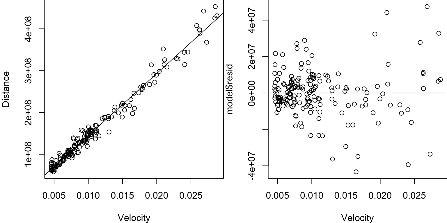
Ideally, the residuals should look randomly and evenly scattered around the \(y=0\) line.
This residual plot shows that:
- The relationship may not be linear (evidence of a U-shape?).
- The error variance may not be constant (appears to be increasing with \(x_i\)).
What about Normality of the Errors?
Don’t try to eyeball it! A quantile-quantile (Q-Q) plot is more reliable.
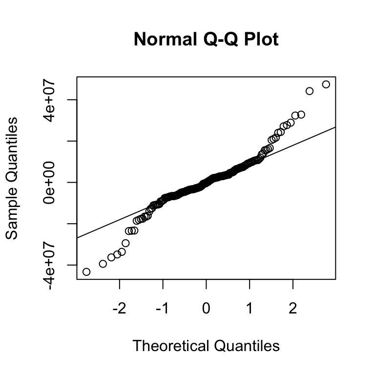
Q-Q Plot
If the errors were normal, the residuals should fall along the line.
Because they do not, there is evidence that the errors are not normal.
What about Independence?
Because we only observe one realization of each residual, it is not possible to test for independence.
Even if it were, the residuals are not independent because they all depend on the same \(\hat\alpha\) and \(\hat\beta\):
- \(e_i = Y_i - (\hat\alpha + \hat\beta x_i)\)
- \(e_j = Y_j - (\hat\alpha + \hat\beta x_j)\).
One common heuristic is to plot the residuals against their order in the data set (sometimes, the data is ordered in a way that reveals nonindependence).
Residuals vs. Order
Recap
- The linear regression model assumes the data are generated from \(Y_i = \alpha + \beta x_i + \epsilon_i\), where \(\epsilon_i\) are i.i.d. \(\text{Normal}(0, \sigma^2)\).
- In this model, the MLEs are the least-squares estimates.
- \(\hat\beta \sim \text{Normal}\left(\beta, \frac{\sigma^2}{\sum_{i=1}^n (x_i - \bar x)^2}\right)\).
- To check model assumptions, we use the residuals \(e_i = Y_i - (\hat\alpha + \hat\beta x_i)\) as a proxy for the errors \(\epsilon_i\) and examine the residual plot and Q-Q plot.
Next time: Using this model to do inference (tests, intervals).