Goodness of Fit and ANOVA

Stats 203

Stanford University

ANOVA Decomposition

Sums of Squares

Three quantities that measure variability in the data:

\[ \begin{align} \text{SST} &= \sum_{i=1}^n (Y_i - \bar{Y})^2 & &\text{(Total Sum of Squares)} \\[6pt] \text{SSM} &= \sum_{i=1}^n (\hat{Y}_i - \bar{Y})^2 & &\text{(Model Sum of Squares)} \\[6pt] \text{SSE} &= \sum_{i=1}^n (Y_i - \hat{Y}_i)^2 & &\text{(Error Sum of Squares)} \end{align} \]

• SST measures total variability in \(Y\) around its mean \(\bar{Y}\).
• SSM measures variability in \(Y\) explained by the model.
• SSE measures remaining (unexplained) variability — we already knew this one!

ANOVA Decomposition

We can decompose the total variability into explained and unexplained variability:

\[ \text{SST} = \text{SSM} + \text{SSE}. \]

This decomposition is critical to the Analysis of Variance (ANOVA).

The proof is by the Pythagorean Theorem.

Recall: \(\hat{\bf Y} = P_{\mathrm{span}({\bf 1},\,{\bf x})}\,{\bf Y}\).

ANOVA Decomposition

We can decompose the total variability into explained and unexplained variability:

\[ \text{SST} = \text{SSM} + \text{SSE}. \]

This decomposition is critical to the Analysis of Variance (ANOVA).

The proof is by the Pythagorean Theorem.

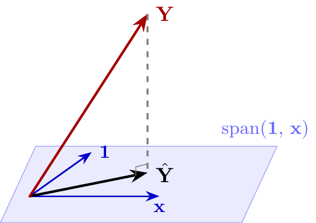
We can also project \({\bf Y}\) onto \({\bf 1}\):

\[ P_{\text{span}({\bf 1})} {\bf Y} = \bar Y {\bf 1}. \]

ANOVA Decomposition

We can decompose the total variability into explained and unexplained variability:

\[ \text{SST} = \text{SSM} + \text{SSE}. \]

This decomposition is critical to the Analysis of Variance (ANOVA).

The proof is by the Pythagorean Theorem.

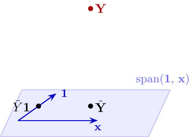
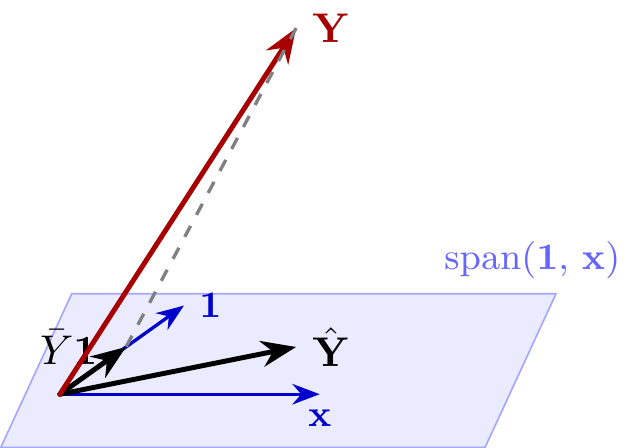
Let’s replace the vectors by points for simplicity.

ANOVA Decomposition

We can decompose the total variability into explained and unexplained variability:

\[ \text{SST} = \text{SSM} + \text{SSE}. \]

This decomposition is critical to the Analysis of Variance (ANOVA).

The proof is by the Pythagorean Theorem.

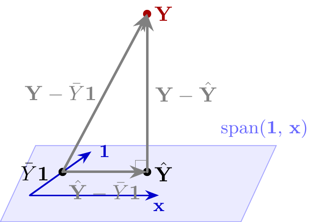
Now we have another right triangle!

\[ {\small ||{\bf Y} - \bar{Y}\mathbf{1}||^2 = || \hat{\mathbf{Y}} - \bar{Y} \mathbf{1} ||^2 + || {\bf Y} - \hat{\mathbf{Y}} ||^2. } \]

ANOVA Decomposition

\[ \begin{align} \underbrace{||{\bf Y} - \bar{Y}\mathbf{1}||^2}_{\text{SST}} &= \underbrace{|| \hat{\mathbf{Y}} - \bar{Y} \mathbf{1} ||^2}_{\text{SSM}} + \underbrace{|| {\bf Y} - \hat{\mathbf{Y}} ||^2}_{\text{SSE}}. \end{align} \]

The only thing left to prove is that \(\hat{\mathbf{Y}} - \bar{Y} \mathbf{1}\) is orthogonal to \({\bf Y} - \hat{\mathbf{Y}}\) so that the Pythagorean Theorem applies.

Coefficient of Determination

How do we measure how well a model fits?

Coefficient of Determination

The coefficient of determination is \[ \frac{\text{SSM}}{\text{SST}}, \] the fraction of total variability in \(Y\) explained by the model.

By the ANOVA decomposition, we can also write this as \[ 1 - \frac{\text{SSE}}{\text{SST}}. \]

Coefficient of Determination for Simple Linear Regression

Theorem. \(\displaystyle\frac{\text{SSM}}{\text{SST}} = r^2\), where \(r\) is the sample correlation between \(x\) and \(Y\).

Remarks

Because it is equivalent to \(r^2\) in simple linear regression, the coefficient of determination is known as \[ R^2 \overset{\text{def}}{=} 1 - \frac{\text{SSE}}{\text{SST}}. \]

It can be used to measure the fit of any model that predicts \(Y\) (e.g., \(k\)-nearest neighbors, decision trees).

• \(R^2\) is the same as \(\frac{\text{SSM}}{\text{SST}}\) for linear regression, but not necessarily for other models.
• \(R^2\) cannot be negative for linear regression, but may be for other models.

ANOVA for Simple Linear Regression

The \(F\)-test

In the Analysis of Variance (ANOVA), we test the hypothesis \[ H_0: \beta = 0 \] by comparing variances: \(\text{SSM}\) vs. \(\text{SSE}\).

If their ratio \[ F = \frac{\text{SSM} / 1}{\text{SSE} / (n - 2)} = \frac{\text{MSM}}{\text{MSE}} \] is large, then we reject \(H_0\). This ratio is called the \(F\)-statistic.

Under \(H_0\), the \(F\)-statistic follows the \(F_{1, n-2}\) distribution.

ANOVA Table

The \(\text{SSM}\), \(\text{SSE}\), \(\text{MSM}\), \(\text{MSE}\), and \(F\)-statistic are typically organized in an ANOVA table:

Relationship between \(F\) and \(t\)

We now have two ways of testing \(H_0: \beta = 0\):

• \(F = \frac{\text{MSM}}{\text{MSE}}\)
• \(t = \frac{\hat\beta}{\text{SE}[\hat\beta]}\)

How do the two tests compare?

Recap

• ANOVA Decomposition: \(\text{SST} = \text{SSM} + \text{SSE}\), proven geometrically via the Pythagorean theorem.
• \(R^2 = r^2\): The fraction of variance explained equals the square of the correlation.
• \(F\)-test: \(F = \dfrac{\text{SSM}/1}{\text{SSE}/(n-2)} \sim F_{1,\,n-2}\) under \(H_0: \beta = 0\).
• For simple linear regression, \(F = t^2\) — the \(F\)-test and \(t\)-test are equivalent.