---
jupytext:
formats: lectures//ipynb,jupyterbook/lectures//md:myst,lectures//Rmd
text_representation:
extension: .md
format_name: myst
format_version: 0.13
jupytext_version: 1.16.7
kernelspec:
display_name: R
language: R
name: ir
---
# Probability
## Download
- [HTML](http://www.stanford.edu/class/stats60/slides/Probability.html)
- [Rmd](http://www.stanford.edu/class/stats60/slides/Probability.Rmd)
- [PDF](http://www.stanford.edu/class/stats60/slides/Probability.pdf)
+++
## Outline
- Frequency as probability
- Rules of probability
- Opposite rule: complements
- Multiplication rule & conditional probability
- Rule of total mass
- Addition rule
- Reading: Chapters 13 & 14 of [Freedman, Pisani and Purves](https://www.amazon.com/Statistics-4th-David-Freedman/dp/8130915871?tag=googhydr-20&source=dsa&hvcampaign=books&gclid=Cj0KCQiA-aK8BhCDARIsAL_-H9ltLmjPLPVAglqzQZM1gPfjhupPL9mvOZfcJc8U57zCCb3aV3Bl7Q0aApTHEALw_wcB)
+++
---
## Probability
### Frequency definition of chances
- If you flip a fair coin many times, the long-run proportion of heads will be 50%.
- Rolling a fair 6-sided die,
will result in a long-run proportion of 1’s of
$$1/6=16 \frac{2}{3}\%.$$
```{code-cell} r
:webr: true
coin_tosses = sample(c('H', 'T'), 10000, replace=TRUE)
mean(coin_tosses == 'H')
die_rolls = sample(1:6, 10000, replace=TRUE)
mean(die_rolls == 1)
```
## Some rules of probability
- *Range of values:* Chances are between 0 % and 100 % (i.e. between 0 and 1).
- *Opposites:* The chance of something equals 100 % minus the chance of the opposite thing.
### Example
The chance of not getting a 1 when rolling a die is
$$
1 - \frac{1}{6} = 83.33\%
$$
---
+++
## Drawing marbles from a box
- Box #1 (`large`) :30 blue, 20 red
- Box #2 (`small`): 3 blue, 2 red
- If you have to draw a blue marble to win, which box would you choose?
```{code-cell} r
:webr: true
large = c(rep('B', 30), rep('R', 20))
small = c(rep('B', 3), rep('R', 2))
```
- They both have the same chance of winning when drawing 1 marble: 0.6
## With or without replacement?
- When drawing one marble, the important number was
$$\frac{\# \ \text{blue marbles}}{\# \ \text{marbles}} = 60\%$$
- What if you draw 5 marbles with replacement?
- Without replacement?
+++
---
## Chances of winning with replacement
- We will see that the chances of winning are
$$
1 - \left(\frac{2}{5}\right)^5
$$
- The fraction $(2/5)^5$ is the chance that we pick 5 red marbles in a row.
## Sampling without replacement
* If drawing without replacement, `small` will be easier to win.
* We’re even guaranteed to win with `small`. **Why?**
---
+++
## Example
- Suppose our experiment consists of drawing a ticket out of a hat with 20
tickets numbered 1 to 20 in it. We are going to draw 3 tickets.
- Describe the hat after each draw if we draw **with replacement.**
What are the possible outcomes of the experiment?
Before and after each draw, the hat has 20 tickets in it.
The possible outcomes are triples of numbers from 1 to 20:
(1,1,4),(2,3,4), etc.
- Describe the hat after each draw if we draw *without replacement*.
What are possible outcomes of the experiment?
After the first draw, the hat has 19 tickets in it,
after the second 18, and after the third 17.
The possible outcomes are all triples of numbers from
1 to 20 but there can be no ties: (1,1,4) is impossible.
+++
---
## Conditional probability
* Observing some information can *change* the chances of something.
* We already saw this in the marble example. If drawing without
replacement, suppose the first draw was red. What are the chances a
blue marble is drawn on the second draw?
* What if we draw with replacement?
* In this examples, we are *given*
that the first draw was red. These chances are *conditioned*
on knowing the first draw was red.
---
+++
## Multiplication rule
**The chance that two things will both happen equals the chance that the
first will happen, multiplied by the chance that the second will
happen *given* the first has happened.**
### Chance of winning with when drawing twice
- Winning is the opposite of losing, so let's compute the chance of losing when drawing twice, starting with `small`.
- The chances of losing when drawing twice with `small` are
$$
\frac{2}{5} \cdot \frac{1}{4} = 0.1
$$
- The chances of losing when drawing twice with `large` are
$$
\frac{20}{50} \cdot \frac{19}{49} = 0.155
$$
+++
---
## Mathematical notation
* "winning when drawing twice from `small`" is called an *event*
;
* "first draw from `small` is red" and "second draw with replacement from `small` is blue" are also events;
* We usually write $P$ for "chances". For an event $E$
$$ P(E) = \text{chances $E$ occurs}. $$
* Conditional probability of an event $A$ given $B$, i.e.
the chances $A$ occurs given $B$ occurs, is
written as
$$
P(A \vert B).
$$
- Multiplication rule can be written as
$$P(A \, \text{and} \, B) = P(A \cap B) = P(A \vert B) * P(B). $$
---
+++
## Rule of total mass
* The chances of *something* occuring are 100%.
* Example: when we drew marbles, the chances we draw a marble whose color is blue or red is 100 %.
* In mathematical notation, we often use $S$ for "something" or the **sample space**
$$P(S) = 100\% \qquad (= 1)$$
* What is the sample space in our marbles example for any particular draw?
+++
---
## Examples: sample space
- What is the sample space if the experiment is to draw 3 balls without replacement
from the small box?
- What if we draw them with replacement?
---
+++
## Example for the rule of total mass
- When drawing from `small` without replacement, we will draw a blue ball within the first three draws.
$$P(\text{one of the first three balls is blue}) = 100 \%$$
- Let's verify the rule of total mass
$$\begin{aligned}
P(\text{first blue ball is on 1st draw }) &= \frac{3}{5} \\
P(\text{first blue ball is on 2nd draw}) &= \frac{2}{5} \times \frac{3}{4} = \frac{3}{10} \\
P(\text{first blue ball is on 3rd draw}) &= \frac{2}{5} \times \frac{1}{4} = \frac{1}{10} \\
\end{aligned}$$
- Summing the probablities $$\frac{3}{5} + \frac{3}{10} +
\frac{1}{10} = 1.$$
+++
---
## Addition rule
**When can we add probabilities of different events?**
- We can add probabilities of events when the events are **disjoint**
or **mutually exclusive**
### Example
- When rolling a die, the events $E_1= \text{roll is 4}$ ,
$E_2=\text{roll is 3}$ are mutually exclusive because the result of
the roll cannot be 4 and 3 simultaneously.
- Therefore
$$
P(\text{roll is 3 or 4}) = \frac{1}{6} + \frac{1}{6} = \frac{1}{3}.
$$
---
+++
## Mutually exclusive events
+++
---
## Non-mutually exclusive events
## Addition rule
- If the events $E_1, E_2$ are mutually exclusive, then
$$ P(E_1 \ \text{or} \ E_2 \ \text{occurs}) = P(E_1) + P(E_2).$$
- This rule works for more than two: if $[E_1, \dots, E_n]$ are mutually exclusive, then
$$ P(E_1 \ \text{or} \ E_2 \ \text{or} \ \dots \ \text{or} \ E_n) = \sum_{i=1}^nP(E_i).$$
- We often write "$E_1$ or $E_2$" as $E_1 \cup E_2$ and
"$E_1$ and $E_2$" as $E_1 \cap E_2$.
- The events $E_1, E_2$ are mutually exclusive if $E_1 \cap E_2$ is empty.
- From a Venn diagram, we can deduce the general form of the addition rule
$$P(E_1 \cup E_2) = P(E_1) + P(E_2) - P(E_1 \cap E_2).$$
- There are also rules that involve more than 2 events.
## Three events
$$
\begin{aligned}
P(E_1 \cup E_2 \cup E_3) &= P(E_1) + P(E_2) + P(E_3) \\
& - P(E_1 \cap E_2) - P(E_1 \cap E_3) - P(E_2 \cap E_3) \\
& + P(E_1 \cap E_2 \cap E_3)
\end{aligned}
$$
---
+++
## A more complicated Venn diagram: four events
## A simple bound on probabilities
- Because chances (or probabilities) are non-negative
we can see that
$$
P(E_1 \cup E_2) \leq P(E_1) + P(E_2)
$$
- Works for many events as well:
$$
P\left(\cup_{i=1}^n E_i \right) \leq \sum_{i=1}^n P(E_i).
$$
## Example
- Google says there is a 40% chance of rain on Friday, a 10% chance of rain on Saturday and a 0% chance of rain on Sunday.
- Google may be wrong about these chances! BUT, if Google's weather predictions follows the rules of probability we should expect it to say
$$
P(\text{rain on at least one of Friday, Saturday or Sunday}) \leq 50%.
$$
### Bound not always useful
- Google predicts 100% chance of precipitation on Tuesday, 10% on Wednesday and 80% on Thursday.
- There is at most 190% chance of rain on one of Tuesday, Wednesday or Thursday.
- BUT, we know there is at most a 100% chance of rain on one of Tuesday, Wednesday or Thursday.
+++
---
## Do probabilities have to be *real*?
- Our previous example used Google's estimate of rain.
- Their forecast team may or may not be good. They are likely somewhat incorrect.
- BUT, their team probably has its own way it computes probabilities.
- We used the rules of probability to say something about chances of rain on the weekend.
### Moral: the rules of probability are math: they describe a (consistent) way of assigning "chances" to events.
---
+++
## Different probabilities, same sample space
- In tossing a coin once, the sample space is $\{\text{head, tail}\}$.
- We will typically assume $P(\text{head})=P(\text{tail})=50%$.
- There are weighted coins out there, for which $Q(\text{head})$ might be 55% (so $Q(\text{tail})$ is 45%). We use the letter
$Q$ because it is a different way of computing chances than $P$.
- **What if we didn't know whether a coin is fair or weighted? How might we decide?**
+++
---
## Multiplication rule & independence
- Intuitively, an event $A$ is independent of $B$ if given $B$, the odds of $A$ are unaffected.
- In mathematical notation, this would be
$$P(A \vert B)=P(A)$$
- If this is true, we say $A$ and $B$ are *independent*.
- Otherwise, $A$ and $B$ are *dependent*.
- The multiplication rule, combined with independence tells us
$$P(A \cap B) = P(A \vert B) * P(B) = P(A) * P(B).$$
## Example for independence
Let's go back to drawing marbles from a box.
- When drawing marbles *with replacement*
the events
$$\begin{aligned}
A &= \text{first draw is red} \\
B &= \text{second draw is blue}
\end{aligned}$$
are *independent*
- We can even conclude that the draws are independent in this case.
- When drawing *without replacement*
the events $A$ and $B$ are dependent. **Show this.**
- We know know that when drawing *with replacement* the probability of drawing 5 red balls in a row is
$$
\left(\frac{2}{5}\right)^5
$$
---
+++
## Counting and probability
- When performing an experiment (drawing a sample) where each outcome is equally likely, we can compute probabilities by counting.
- Example: when rolling two dice, what is the probability of obtaining a sum of 9?
- For such experiments $$P(E) = \frac{\# E}{\# S}$$ where $S$ is the set of all possible outcomes (our *sample space*).
## Counting example: rolling a pair of dice
- ** What is the sample space?**
| Die 1 \ Die 2 | 1 | 2 | 3 | 4 | 5 | 6 |
|---|---|---|---|---|---|---|
| **1** | (1,1) | (1,2) | (1,3) | (1,4) | (1,5) | (1,6) |
| **2** | (2,1) | (2,2) | (2,3) | (2,4) | (2,5) | (2,6) |
| **3** | (3,1) | (3,2) | (3,3) | (3,4) | (3,5) | (3,6) |
| **4** | (4,1) | (4,2) | (4,3) | (4,4) | (4,5) | (4,6) |
| **5** | (5,1) | (5,2) | (5,3) | (5,4) | (5,5) | (5,6) |
| **6** | (6,1) | (6,2) | (6,3) | (6,4) | (6,5) | (6,6) |
+++
---
## What are the chances the sum will be equal to 9?
| Die 1 \ Die 2 | 1 | 2 | 3 | 4 | 5 | 6 |
|---|---|---|---|---|---|---|
| **1** | 2 | 3 | 4 | 5 | 6 | 7 |
| **2** | 3 | 4 | 5 | 6 | 7 | 8 |
| **3** | 4 | 5 | 6 | 7 | 8 | 9 |
| **4** | 5 | 6 | 7 | 8 | 9 | 10 |
| **5** | 6 | 7 | 8 | 9 | 10 | 11 |
| **6** | 7 | 8 | 9 | 10 | 11 | 12 |
- There are 4 outcomes whose sum is 9. Therefore, the chances are $\frac{4}{36}=\frac{1}{9}$.
## What are the chances the sum will be greater than or equal to 7?
| Die 1 \ Die 2 | 1 | 2 | 3 | 4 | 5 | 6 |
|---|---|---|---|---|---|---|
| **1** | 2 | 3 | 4 | 5 | 6 | 7 |
| **2** | 3 | 4 | 5 | 6 | 7 | 8 |
| **3** | 4 | 5 | 6 | 7 | 8 | 9 |
| **4** | 5 | 6 | 7 | 8 | 9 | 10 |
| **5** | 6 | 7 | 8 | 9 | 10 | 11 |
| **6** | 7 | 8 | 9 | 10 | 11 | 12 |
- There are 21 outcomes whose sum is greater than or equal to 7. Therefore, the chances are $\frac{21}{36}=\frac{7}{12}$.
## What are the chances the sum will be less than 7?
- The chances that the sum is greater than or equal to 7 are $\frac{7}{12}$.
Therefore, by the "opposite" rule, the chances are chances are
$$1−\frac{7}{12}=\frac{5}{12}.$$
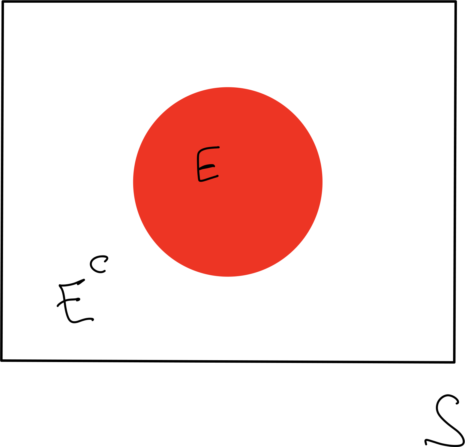
## Complement of an event
- Formally, the "opposite" rule is the rule of *complements*.
- We write the complement of an event $E$ as $E^c$
$$P(\text{not} \, E) = P(E^c).$$
- The rule of *complements*
says
$$P(E^c) = 1 - P(E)$$
---
+++
## An event $E$ and its complement $E^c$
+++
---
## Properties of complements
* For any event $E$, $E$ and $E^c$ are mutually exclusive.
* For any event $E$, $S = E \cup E^c$.
* For any two events $A, B$
$$\begin{aligned}
B &= B \cap S \\
&= B \cap (A \cup A^c) \\
&= (B \cap A) \cup (B \cap A^c)
\end{aligned}$$
where $B \cap A$ and $B \cap A^c$ are mutually exclusive (i.e. disjoint).
* Therefore,
$$
P(B) = P(B \cap A) + P(B \cap A^c).
$$
---
+++
## Using complements to decompose
* For the `small` box, if we draw with replacement, what are the chances it will take less than 6 draws to draw 1st blue marble?
* If $E$={takes less than 6 draws to draw 1st blue marble}, then
$$\begin{aligned}
E^c &=\{\text{takes 6 or more draws to draw 1st blue marble}\} \\
&=\{\text{first 5 draws are red}\} \\
\end{aligned}$$
* By independence,
$$
P(\text{first 5 draws are red}) = \left(\frac{2}{5}\right)^5
$$
* Therefore,
$$P(\text{takes less than 6 draws to draw 1st blue marble}) = 1 - \left(\frac{2}{5}\right)^5 = 99\%$$
## Using complements 2nd example
- For the `small box` suppose we draw without replacement and want to compute
$$
P(\text{2nd marble is blue})
$$
- We know
$$
\begin{aligned}
P(\text{1st marble is red, 2nd marble is blue}) &= \frac{2}{5} * \frac{3}{4} \\
P(\text{1st marble is not red, 2nd marble is blue}) &= P(\text{1st marble is blue, 2nd marble is blue}) \\
\frac{3}{5} * \frac{2}{4} \\
\end{aligned}
$$
- Therefore
$$
P(\text{2nd marble is blue}) = \frac{2}{5} * \frac{3}{4} + \frac{3}{5} * \frac{2}{4} = \frac{3}{5}
$$
+++
---
## Bayes' rule
- Credited to [Reverend Thomas Bayes](http://en.wikipedia.org/wiki/Thomas_Bayes)
- Given two events $A$ and $B$
$$\begin{aligned}
P(A \vert B) &= \frac{P(B \, \text{and} \, A)}{P(B)} \\
&= \frac{P(A \cap B)}{P(B)} \\
&= \frac{P(B \vert A)\times P(A)}{P(B)}
\end{aligned}$$
- The formula is a direct consequence of the multiplication rule.
---
+++
### Alternate version of Bayes' rule
- By the properties of complements
$$\begin{aligned}
P(B) &= P(B \cap A) + P(B \cap A^c) \\
&= P(B \vert A) \times P(A) + P(B \vert A^c) \times P(A^c)
\end{aligned}$$
- Other versions of Bayes' rule
$$\begin{aligned}
P(A \vert B) &= \frac{P(B \vert A) \times P(A)}{P(B \vert A) \times P(A) + P(B \vert A^c) \times P(A^c) } \\
&= \frac{P(B \cap A)}{P(B \cap A) + P(B \cap A^c)} \\
\end{aligned}$$
+++
---
## Drawing marbles without replacement from `small` box using Bayes' rule
- Let
$$\begin{aligned}
A&=\{\text{draw a red marble on first draw}\} \\
B&=\{\text{draw a blue marble on second draw}\} \\
\end{aligned}$$
- **Compute $P(A \vert B)$.**
* What do we know?
$$\begin{aligned}
P(A) &= \frac{2}{5} \\
P(B \vert A) &= \frac{3}{4} \\
\end{aligned}$$
---
+++
- We need $$P(B) = P(B \vert A) \times P(A) + P(B \vert A^c) \times P(A^c).$$
- Note that $A^c=\{\text{draw a blue marble on first draw}\}$.
- We know
$$\begin{aligned}
P(A^c) &= \frac{3}{5} \\
P(B \vert A^c) &= \frac{1}{2} \\
\end{aligned}$$
- Therefore,
$$\begin{aligned}
P(B) &= \frac{3}{4} \times \frac{2}{5} + \frac{1}{2} \times \frac{3}{5} = \frac{3}{10} \\
P(A \vert B) &= \frac{ \frac{3}{4} \times \frac{2}{5}}{\frac{3}{4} \times \frac{2}{5} + \frac{1}{2} \times \frac{3}{5}} = \frac{1}{2}
\end{aligned}$$
## Using alternate form
- Earlier, we computed $P(\text{2nd marble is blue}) = P(B)$ as
$$
P(B \cap A) + P(B \cap A^c) = \frac{2}{5} * \frac{3}{4} + \frac{3}{5} * \frac{2}{4}
$$
- So,
$$
P(A|B) = \frac{\frac{2}{5} * \frac{3}{4}}{\frac{2}{5} * \frac{3}{4} + \frac{3}{5} * \frac{2}{4}}
$$
+++
---
## Diagnostic testing
- Suppose a patient from some population is tested for a disease based on some diagnostic test.
- The prevalence of the disease is 0.1% in the population.
- If a patient has the disease, the test result is positive with probability 95 %. (*True positive*
)
- If a patient does not have the disease, the test result is positive with probability 1 %. (*False positive*
).
- What is the probability a patient has the disease given a positive test result? What if the false positive rate were 0.1%?
---
+++
- Let
$$\begin{aligned}
D &= \{\text{patient has disease}\} \\
T^+ &= \{\text{test result is positive}\} \\
\end{aligned}$$
- We are given
$$\begin{aligned}
P(D) &= 0.001 \\
P(T^+ \vert D) &= 0.95 \\
P(T^+ \vert D^c) &= 0.01 \\
\end{aligned}$$
- We want to compute $P(D \vert T^+)$.
- By Bayes’ theorem
$$\begin{aligned}
P(D \vert T^+) &= \frac{P(T^+ \vert D) \times P(D)}{P(T^+ \vert D) \times P(D) + P(T^+ \vert D^c) \times P(D^c)} \\
&= \frac{0.95 \times 0.001}{0.95 \times 0.001 + 0.01 \times 0.999} \\
&= 8.7 \%
\end{aligned}$$
+++
---
### Changing the false positive rate
* If the test makers improve their false positive rate to 0.001 then
$$\begin{aligned}
P(D \vert T^+)
&= \frac{0.95 \times 0.001}{0.95 \times 0.001 + 0.001 \times 0.999} \\
&= 48.7 \%
\end{aligned}$$