CCA (Canonical Correlation Analysis)
Canonical correlation analysis
For a data matrix \(X \in \mathbb{R}^{n \times p}\) with \(X_i \overset{IID}{\sim} F\) , PCA and Factor Analysis can be thought of as models / decompositions of
\[
\Sigma = \text{Var}_F(X)
\]
Canonical correlation analysis deals with pairs \(\mathbb{R}^p \times \mathbb{R}^q \ni (X_i, Y_i) \overset{IID}{\sim} F\) and models / decomposes the cross-covariance matrix
\[
\text{Var}_F(X,Y) = \begin{pmatrix} \Sigma_{XX} & \Sigma_{XY} \\ \Sigma_{YX} & \Sigma_{YY} \end{pmatrix}.
\]
\[
\text{maximize}_{(a,b): a^T\Sigma_{XX}a \leq 1, b^T\Sigma_{YY}b \leq 1} a^T\Sigma_{XY}b
\]
Example from here
\(X\) : psychological variables: (Control, Concept, Motivation)
\(Y\) : academic + sex: (Read, Write, Math, Science, Sex)
= read.csv ("https://stats.idre.ucla.edu/stat/data/mmreg.csv" )head (mm)
  locus_of_control self_concept motivation read write math science female
1            -0.84        -0.24       1.00 54.8  64.5 44.5    52.6      1
2            -0.38        -0.47       0.67 62.7  43.7 44.7    52.6      1
3             0.89         0.59       0.67 60.6  56.7 70.5    58.0      0
4             0.71         0.28       0.67 62.7  56.7 54.7    58.0      0
5            -0.64         0.03       1.00 41.6  46.3 38.4    36.3      1
6             1.11         0.90       0.33 62.7  64.5 61.4    58.0      1
Substituting \(u=\Sigma_{XX}^{1/2}a, v=\Sigma_{YY}^{1/2}v\) we see that \((u, v)\) solve
\[
\text{maximize}_{(u,v): \|u\|_2 \leq 1, \|v\|_2 \leq 1} u^T\Sigma_{XX}^{-1/2}\Sigma_{XY}\Sigma_{YY}^{-1/2}v
\]
So \(u=U[,1]\) and \(v=V[,1]\) are leading left and right singular vectors of \(\Sigma_{XX}^{-1/2}\Sigma_{XY}\Sigma_{YY}^{-1/2}= U \rho V^T\) with \(\rho=\text{diag}(\rho_1, \dots,\rho_q)\) .
Achieved maximal correlation value is the leading singular value \(\rho_1\) .
Practically speaking, can find SVD by eigendecomposition of the symmetric matrix
\[
\Sigma_{XX}^{-1/2}\Sigma_{XY}\Sigma_{YY}^{-1}\Sigma_{YX} \Sigma_{XX}^{-1/2} = U\rho^2 U'
\]
Loadings \(a=\Sigma_{XX}^{-1/2}u, b=\Sigma_{YY}^{-1/2}v\) determine first canonical variates \((a^TX, b^TY)\) with
\[
\text{Var}_F(a^TX) = \text{Var}_F(b^TY) = 1, \qquad \text{Cov}_F(a^TX, b^TY) = \rho_1.\]
Second canonical variate problem:
\[
\text{maximize}_{(a_2,b_2): a_2^T\Sigma_{XX}a_2 \leq 1, b_2^T\Sigma_{YY}b_2 \leq 1} a_2^T\Sigma_{XY}b_2
\]
subject to \(\text{Cov}_F(a_1^TX,a_2^TX)=\text{Cov}_F(b_1^TY, b_2^TY)=0\) .
Not hard to see that \(a_2=\Sigma_{XX}^{-1/2}U[,2], b_2=\Sigma_{YY}^{-1/2}V[,2]\) .
Realized correlation is \(\rho_2\) .
Continuing
\[
A = \Sigma_{XX}^{-1/2}U, \qquad B=\Sigma_{YY}^{-1/2}V.
\]
Final form of covariance matrix
\[
\text{Cov}_F(A'X, B'Y) = \begin{pmatrix} I & R \\
R^T & I \end{pmatrix}
\]
Assuming non-singular covariances, when \(p > q\)
\[
R = \begin{pmatrix} \rho \\ 0 \end{pmatrix}
\]
transposing when \(p \leq q\) .
Generative model
\[
\begin{aligned}
\check{Z} & \sim N(0, I_q) \\
\epsilon_X & \sim N(0, I_p) \\
\epsilon_Y & \sim N(0, I_q) \\
Z_Y &= \sqrt{1 - \rho} \cdot \epsilon_Y + \sqrt{\rho} \cdot \check{Z} \\
Z_X[1:p] &= \sqrt{1 - \rho} \cdot \epsilon_X[1:q] + \sqrt{\rho} \cdot \check{Z} \\
Z_X[(q+1):p] &= \epsilon_X[(q+1):p] \\
X &= \Sigma_{XX}^{1/2} \textcolor{red}{\bar{U}} Z_X \\
Y &= \Sigma_{YY}^{1/2} \textcolor{red}{V} Z_Y
\end{aligned}
\]
Sample version
Simply replace \(\Sigma\) with \(\widehat{\Sigma}\) .
Under non-degeneracy assumptions, matrices \(\widehat{\Sigma}_{XX}\) and \(\widehat{\Sigma}_{YY}\) will be invertible if \(n > \text{max}(q,p)\) .
As in PPCA, Bach & Jordan (2006) show that sample estimates are MLE for this generative model
\(\implies\) could use likelihood to choose rank…
library (CCA)= mm[,1 : 3 ]= mm[,- c (1 : 3 )]= CCA:: cc (X, Y)names (CCA_mm)
[1] "cor" "names" "xcoef" "ycoef" "scores"
Checking CCA solution
= cov (mm)[1 : 3 ,4 : 8 ]t (CCA_mm$ xcoef) %*% crosscov %*% CCA_mm$ ycoef
             [,1]          [,2]          [,3]
[1,] 4.640861e-01  5.599087e-17 -1.930228e-16
[2,] 3.610083e-16  1.675092e-01 -3.725764e-16
[3,] 4.012970e-16 -5.498621e-16  1.039911e-01
                       [,1]       [,2]       [,3]
locus_of_control -1.2538339 -0.6214776 -0.6616896
self_concept      0.3513499 -1.1876866  0.8267210
motivation       -1.2624204  2.0272641  2.0002283
Diagonalizes the \(X\) and \(Y\) subblocks
= cov (mm)[1 : 3 ,1 : 3 ]t (CCA_mm$ xcoef) %*% Xcov %*% CCA_mm$ xcoef
             [,1]          [,2]          [,3]
[1,] 1.000000e+00  2.478633e-16  2.048775e-16
[2,] 3.413977e-16  1.000000e+00 -1.345034e-16
[3,] 2.169002e-16 -1.469862e-16  1.000000e+00
= cov (mm)[4 : 8 ,4 : 8 ]t (CCA_mm$ ycoef) %*% Ycov %*% CCA_mm$ ycoef
              [,1]          [,2]          [,3]
[1,]  1.000000e+00 -1.975726e-16  2.677851e-17
[2,] -1.686276e-16  1.000000e+00 -4.013920e-15
[3,] -1.444754e-17 -4.112697e-15  1.000000e+00
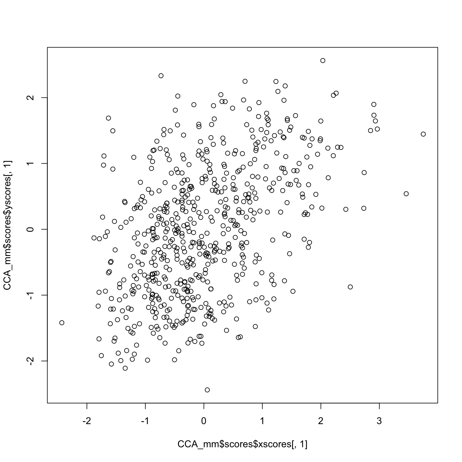
plot (CCA_mm$ scores$ xscores[,1 ], CCA_mm$ scores$ yscores[,1 ])
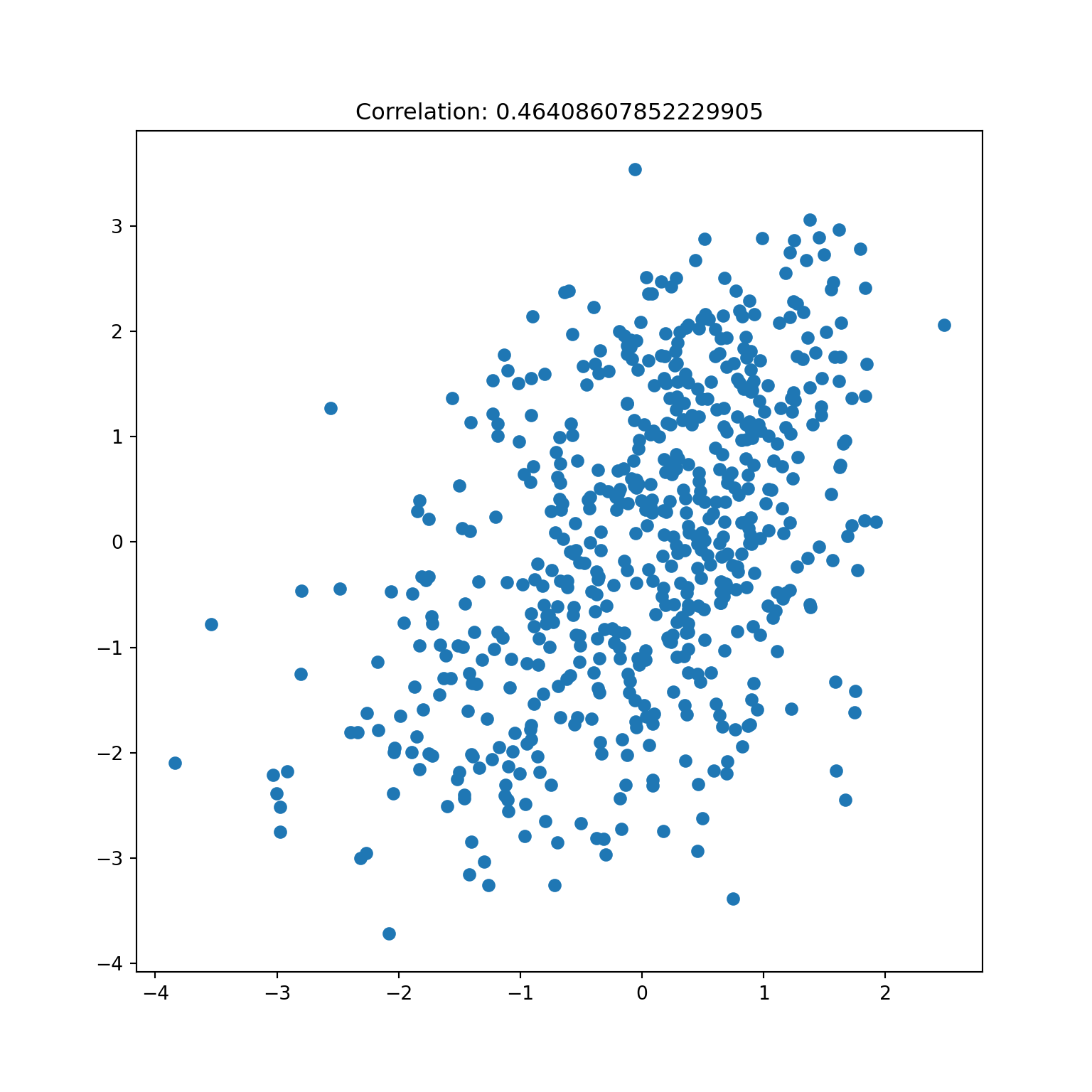
= CCA(n_components= 3 ); = cca.transform(X, Y)
= plt.subplots()0 ], Y_t[:,0 ])f'Correlation: { np. corrcoef(X_t[:,0 ], Y_t[:,0 ])[0 ,1 ]} ' )
= CCA:: cc (scale (X, TRUE , TRUE ), scale (Y, TRUE , TRUE ))cbind (CCA_mm$ cor, CCA_mm_scaled$ cor)
          [,1]      [,2]
[1,] 0.4640861 0.4640861
[2,] 0.1675092 0.1675092
[3,] 0.1039911 0.1039911
lm (CCA_mm$ scores$ xscores[,1 ] ~ CCA_mm_scaled$ scores$ xscores[,1 ])
Call:
lm(formula = CCA_mm$scores$xscores[, 1] ~ CCA_mm_scaled$scores$xscores[,
    1])

Coefficients:
                      (Intercept)  CCA_mm_scaled$scores$xscores[, 1]
                         9.15e-16                           1.00e+00
= matrix (rnorm (9 ), 3 , 3 )= as.matrix (X) %*% A= CCA:: cc (XA, Y)cbind (CCA_mm$ cor, CCA_affine$ cor)
          [,1]      [,2]
[1,] 0.4640861 0.4640861
[2,] 0.1675092 0.1675092
[3,] 0.1039911 0.1039911
lm (CCA_mm$ scores$ xscores[,1 ] ~ CCA_affine$ scores$ xscores[,1 ])
Call:
lm(formula = CCA_mm$scores$xscores[, 1] ~ CCA_affine$scores$xscores[,
    1])

Coefficients:
                   (Intercept)  CCA_affine$scores$xscores[, 1]
                     8.153e-16                      -1.000e+00
Relation to reduced rank regression
For each of \(X\) and \(Y\) , we saw that there are mappings
\[
X \mapsto U^T\Sigma^{-1/2}_{XX}X = A^TX = Z_X, \qquad Y \mapsto V^T\Sigma_{YY}^{-1/2}Y = B^TY = Z_Y
\]
to unitless canonical variates .
These canonical variates drive the correlation between \(X\) and \(Y\) …
Reduced rank regression for rank \(k \leq \text{min}(p, q)\)
Due to affine equivariance, it’s not hard to see that
\[
\hat{Y} = \Sigma_{YY}^{1/2} V[,1:k] \rho[1:k] Z_X[1:k]
\]
Inference: how to test \(\rho_j=0, j \geq k\) ?
Complicated joint densities…
Not too hard under global null \(H_0:\Sigma_{XY}=0\) , though these tests will all look like tests for regression \(Y\) onto \(X\) .
Under global null \(H_0: X \ \text{ independent of} \ Y\) could permute either \(X\) or \(Y\) …
Generalizations
For non-Euclidean data we might featurize either \(X\) , \(Y\) or both.
This idea shows up over and over: given features \(X\) , make new features through a basis expansion (which include the kernel trick ).
We see this in two-sample tests (e.g. in the kernelized versions); linear regression; kernel PCA; etc.
Wherever we form random variables like \(\beta^TX\) , we can replace with \(W=f(X)\) …
Often, methods with richer (i.e. more) features will also feature a regularization term …
Which new features? This is domain dependent…
Kernelized CCA
Given linear spaces of features \({\cal H}_X, {\cal H}_Y\) we might look at
\[
\text{maximize}_{(f, g) \in {\cal H}_X \times {\cal H}_Y: \text{Var}_F(f(X)) \leq 1, \text{Var}_F(g(Y)) \leq 1}
\text{Cov}_F(f(X), g(Y)).
\]
If \({\cal H}_X\) and \({\cal H}_Y\) are RKHS, this is kernelized CCA .
A possible issue?
For kernelized CCA \(\text{max}(\text{dim}({\cal H}_X), \text{dim}({\cal H}_Y)) > n\) the matrix
\[
\widehat{\text{Cov}}_F(f_i(X), f_j(X)) = \widehat{\Sigma}_{f(X),f(X)}
\]
is degenerate so we can’t really form \(\widehat{\Sigma}_{f(X),f(X)}^{-1/2}\) …
Generic RKHS will always have this problem. How to resolve?
Regularized covariance estimate
Let’s just assume that \({\cal H}_X\) is finite dimensional of dimension \(k > n\) and \({\cal H}_Y\) are just the usual linear functions.
We can then just work on the usual CCA with data matrices \(Y\) and \(W=f(X) \in \mathbb{R}^{n \times k}\) .
A simple remedy is to consider instead
\[
\text{maximize}_{(a,b): a^T(\widehat{\Sigma}_{WW}+\epsilon I)a \leq 1, b^T\widehat{\Sigma}_{YY}b \leq 1} a^T\widehat{Cov}_{WY}b
\]
Will require SVD of \((\widehat{\Sigma}_{WW} + \epsilon I)^{-1/2} \widehat{\Sigma}_{WY} \widehat{\Sigma}_{YY}^{-1/2}\) .
Kernelized version
Instead of \(\widehat{\text{Var}}(f(X))\) could use
\[
f \mapsto \widehat{\text{Var}}(f(X)) + \epsilon \|f\|^2_{{\cal H}_X}.
\]
Even simpler (in theory): subsample the “knots” in the kernel (e.g. Snelson & Ghahramani (2005) )
By usual kernel trick, this reduces problem to an \(n\) dimensional problem.
In this case, an eigenvalue problem for \(n \times n\) matrix…
Other covariance regularization
(PMD) Witten et al. (pretends \(\Sigma_{WW}= \kappa I\) )
NOCCO in Fukumizu et al. (uses the regularized covariance operator in RKHS)
Use row/column covariance Allen et al.
Each of these methods boils down to choosing two quadratic forms \(Q_X, Q_Y\) …
Other structure
Restricting to finite dimensions, the first regularized problems morally look like (assuming \(X\) and \(Y\) have been centered)
\[
\text{maximize}_{(a,b): a^TQ_Xa \leq 1, b^TQ_Yb \leq 1} a^TX^TYb
\]
It is often tempting to interpret loadings \((a,b)\) just as in PCA.
For such settings, it is often desirable to impose structure on \((a,b)\) .
Sparse CCA and variants
In bound form: \[
\text{maximize}_{(a,b): a^TQ_Xa \leq 1, b^TQ_Yb \leq 1, \|a\|_1 \leq c_X } a^TX^TYb
\]
In Lagrange form: \[
\text{maximize}_{(a,b): a^TQ_Xa \leq 1, b^TQ_Yb \leq 1} a^TX^TYb - \lambda_X \|a\|_1
\]
Non-negative factors
\[
\text{maximize}_{(a,b): a^TQ_Xa \leq 1, b^TQ_Yb \leq 1, a \geq 0, b \geq 0} a^TX^TYb
\]
Relation to sparse PCA
Corresponds to swapping \(X^TY\) with \(X\) …
A bi-convex problem
The function \((a,b) \mapsto -a^TX^TYb\) is not convex.
Numeric feasibility of solving PCA rests on computability of SVD even though it is not a convex problem.
However, for \(b\) fixed, \(a \mapsto -a^TX^TYb\) is linear, hence convex.
Alternating algorithm: given feasibile initial \((\widehat{a}^{(0)}, \widehat{b}^{(0)})\) we iterate (for \(\ell_1\) bound form above):
\[
\begin{aligned}
\widehat{a}^{(t)} &= \text{argmin}_{a: a^TQ_Xa \leq 1, \|a\|_1 \leq c_1} - a^TX^TY\widehat{b}^{(t-1)} \\
\widehat{b}^{(t)} &= \text{argmin}_{b: b^TQ_Yb \leq 1} - (\widehat{a}^{(t)})^TX^TYb \\
\end{aligned}
\]
Yields an ascent algorithm on objective \((a,b) \mapsto a^TX^TYb\) … often with pretty simple updates.
Deflation not completely obvious, but there are reasonable proposals
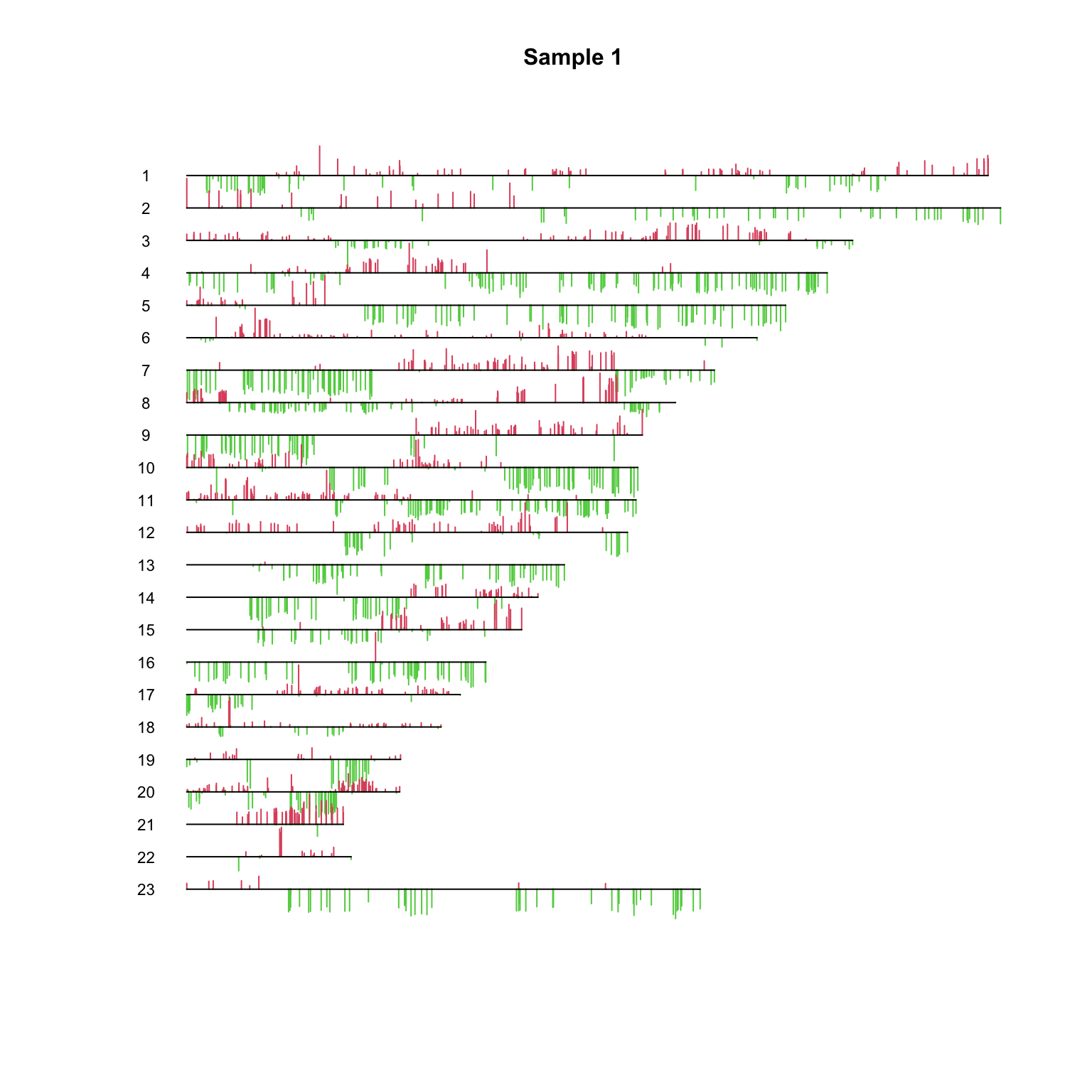
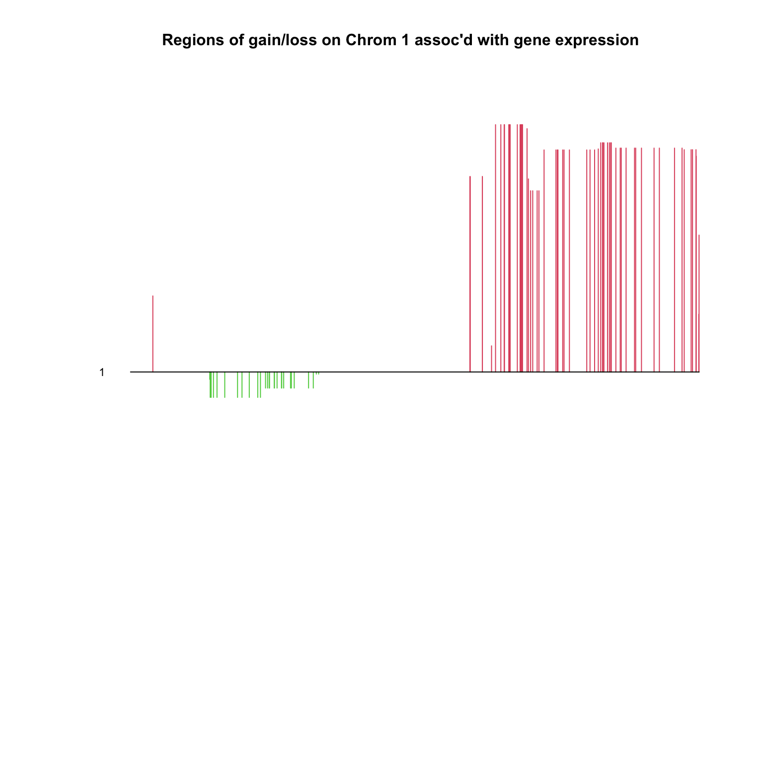
An example with a pretty picture: CGH
An example with a pretty picture: CGH
Dataset breastdata from PMA has both gene expression data (rna) and CGH measurements (dna) on 89 samples.
Our example (which is in PMA package) will just use CGH from chromosome 1: t(dna) is a \(89 \times 136\) matrix and all of t(rna), an \(89 \times 19672\) matrix.
CGH data is modeled as piecewise constant with a (sparse) fused LASSO penalty constraint \[
{\cal P}_{FL}(v) = \|v\|_1 + \alpha \|Dv\|_1 \leq c_v
\] while gene expression is sparse \[
{\cal P}_S(u) = \|u\|_1.
\]
Optimization problem: \[
\text{maximize}_{(u,v): \|u\|_2\leq 1, {\cal P}_S(u) \leq c_u, \|v\|_2 \leq 1, {\cal P}_{FL}(v) \leq c_v} u^TX^TYv
\]
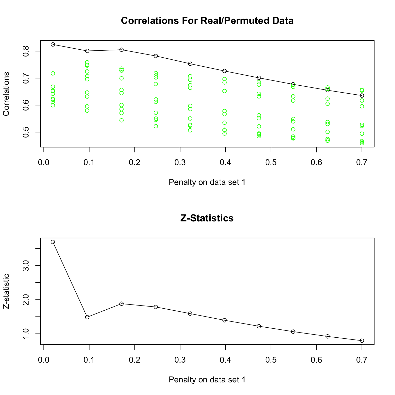
Inevitably, one has to choose tuning parameters…
Authors propose permuting \(X\) and rerunning algorithm while retaining the value of the problem. Parameters are chosen to have smallest p-value .
set.seed (22 )= t (dna)= t (rna)= CCA.permute (x= rna_t,## Run CCA using all gene exp. data, but CGH data on chrom 1 only. z= dna_t[,chrom== 1 ],typex= "standard" ,typez= "ordered" ,nperms= 10 ,penaltyxs= seq (.02 ,.7 ,len= 10 ))
 Permutation  1  out of  10  12345678910
 Permutation  2  out of  10  12345678910
 Permutation  3  out of  10  12345678910
 Permutation  4  out of  10  12345678910
 Permutation  5  out of  10  12345678910
 Permutation  6  out of  10  12345678910
 Permutation  7  out of  10  12345678910
 Permutation  8  out of  10  12345678910
 Permutation  9  out of  10  12345678910
 Permutation  10  out of  10  12345678910
Call: CCA.permute(x = rna_t, z = dna_t[, chrom == 1], typex = "standard",
    typez = "ordered", penaltyxs = seq(0.02, 0.7, len = 10),
    nperms = 10)

Type of x:  standard
Type of z:  ordered
   X Penalty Z Penalty Z-Stat P-Value  Cors Cors Perm FT(Cors) FT(Cors Perm)
1      0.020     0.032  3.694     0.0 0.825     0.641    1.171         0.762
2      0.096     0.032  1.487     0.0 0.801     0.684    1.101         0.845
3      0.171     0.032  1.882     0.0 0.805     0.649    1.113         0.783
4      0.247     0.032  1.786     0.0 0.782     0.623    1.050         0.739
5      0.322     0.032  1.591     0.0 0.753     0.603    0.980         0.706
6      0.398     0.032  1.396     0.0 0.726     0.587    0.921         0.681
7      0.473     0.032  1.221     0.0 0.701     0.574    0.869         0.661
8      0.549     0.032  1.063     0.0 0.677     0.563    0.823         0.644
9      0.624     0.032  0.922     0.2 0.655     0.553    0.784         0.630
10     0.700     0.032  0.796     0.2 0.635     0.546    0.750         0.619
   # U's Non-Zero # Vs Non-Zero
1              12            90
2             267            72
3            1189            71
4            2639            62
5            4329            62
6            6278            61
7            8399            61
8           10860            61
9           13536            61
10          16252            61
Best L1 bound for x:  0.02
Best lambda for z:  0.03178034
What is the \(Z\) -score?
For each permutation, there is a realized value to the optimization problem for each value of the tuning parameter.
Can compute mean and SD over permutation data (for each value of the tuning parameter), yielding a reference distribution.
\(Z\) -score compares observed realized value to the permutation distribution.
Tuning parameter is chosen to maximize the \(Z\) -score.
= CCA (x= rna_t,z= dna_t[,chrom== 1 ], typex= "standard" , typez= "ordered" ,penaltyx= perm.out$ bestpenaltyx,v= perm.out$ v.init, penaltyz= perm.out$ bestpenaltyz,xnames= substr (genedesc,1 ,20 ),znames= paste ("Pos" , sep= "" , nuc[chrom== 1 ]))print (out, verbose= FALSE ) # could do print(out,verbose=TRUE)
Call: CCA(x = rna_t, z = dna_t[, chrom == 1], typex = "standard", typez = "ordered",
    penaltyx = perm.out$bestpenaltyx, penaltyz = perm.out$bestpenaltyz,
    v = perm.out$v.init, xnames = substr(genedesc, 1, 20), znames = paste("Pos",
        sep = "", nuc[chrom == 1]))


Num non-zeros u's:  12
Num non-zeros v's:  90
Type of x:  standard
Type of z:  ordered
Penalty for x: L1 bound is  0.02
Penalty for z: Lambda is  0.03178034
Cor(Xu,Zv):  0.8247056
print (genechr[out$ u!= 0 ]) # which chromosome are the selected genes on
[1] 1 1 1 1 1 1 1 1 1 1 1 1
PlotCGH (out$ v, nuc= nuc[chrom== 1 ], chrom= chrom[chrom== 1 ],main= "Regions of gain/loss on Chrom 1 assoc'd with gene expression" )
Multiple CCA
We had gene expression and CGH data on the same samples.
Can easily conceive of situations where we have yet another type of phenotype.
Given samples from \(X=(X_1, \dots, X_r) \sim F, X_i \in \mathbb{R}^{d_i}\) we can write its covariance as
\[
\text{Var}_F(X) = \begin{pmatrix} \Sigma_{11} & \Sigma_{12} & \dots \\
\Sigma_{21} & \Sigma_{22} & \dots \\
\vdots & \ddots & \dots
\end{pmatrix}
\] with \(\Sigma_{ij} \in \mathbb{R}^{d_i \times d_j}\) .
Forming linear combinations \(a_i^TX_i, a_j^TX_j\) yields
\[
\text{Var}_F(a_1^TX_1,\dots, a_r^TX_r) = \begin{pmatrix} a_1^T\Sigma_{11}a_1 & a_2^T\Sigma_{12}a_2 & \dots \\
a_2^T\Sigma_{21}a_1 & a_2^T\Sigma_{22}a_2 & \dots \\
\vdots & \ddots & \dots
\end{pmatrix} \in \mathbb{R}^{r \times r}
\]
Pick your favorite functional \(\Phi\) of the off-diagonal blocks – try to maximize
\[
\Phi\left(\text{Var}_F(a_1^TX_1,\dots, a_r^TX_r)\right)
\]
subject to \(\text{Var}_F(a_i^TX_i)=1, 1 \leq i \leq r\) .
Examples of \(\Phi\) : sum of off-diagonals; max of off-diagonals…
Covariance can be regularized…
Can impose structure (sparsity, non-negativity, etc.)
Solving the problem? Certainly the sum of off-diagonals is multi-convex…
See Witten and Tibshirani (2009)
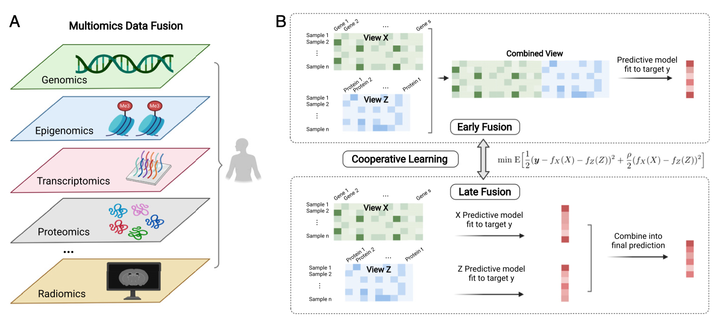
Cooperative learning
The CCA problem is unsupervised (though is related to reduced rank regression…)
In supervised setting, we might have different views (qualitatively different types of data)
Genetic data
Different types of biological assay
Imaging data
\[
\text{minimize}_{f_X, f_Z} \frac{1}{2} \mathbb{E} \left[ \left(Y - f_Z(Z) - f_X(Z) \right) + \frac{\rho}{2}\left(f_X(X) - f_Z(Z)\right)^2 \right]
\]
Underlying generative model (?)
\(X\) , \(Z\) as in the CCA generative model with common variation \(\check{Z}\)
\(Y | \check{Z}, X, Z \sim N(\alpha'\check{Z} + \beta'X + \gamma'Z, \sigma^2)\) with \(\beta\) , \(\gamma\) simple
Supervised target shares some of the same latent variables as \(X\) and \(Z\) …