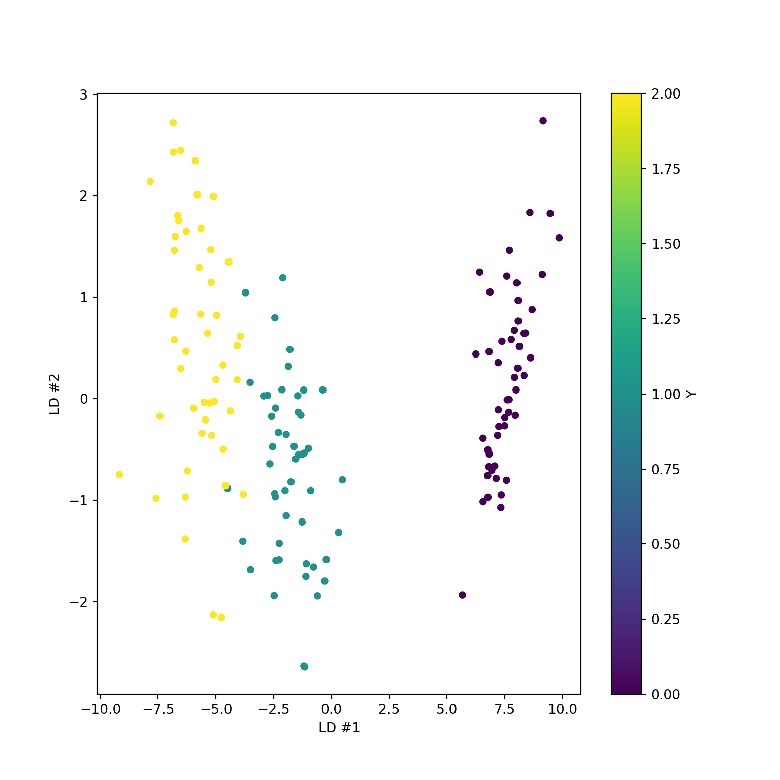
iris = load_iris()
X = iris.data
y = iris.target
lda = LDA()
lda.fit(X, y);
y_pred = lda.predict(X)
print(f"Accuracy: {lda.score(X, y):.2f}")
Accuracy: 0.98
Given \(K\) classes in \(\mathbb{R}^p\), represented as densities \(f_i(x), 1 \leq i \leq K\) we want to classify \(x \in \mathbb{R}^p\).
In other words, partition \(\mathbb{R}^p\) (or other sample space) into subsets \(\Pi_i, 1 \leq i \leq k\) based on the densities \(f_i(x)\).
We’ll focus on classical methods: LDA and generalizations.
LDA is a misnomer: it is a generative classifier rather than discriminative classifier.
\[ x \in \Pi_i \iff i = \text{argmax}_{j} f_j(x)\]
\[ x \in \Pi_i \iff i= \text{argmax}_{j} \pi_j f_j(x).\]
Suppose the sample space is all \(p\)-tuples of integers that sum to \(n\).
Two classes \(f_1 = \text{Multinom}(n, \alpha)\), \(f_2 = \text{Multinom}(n, \beta)\).
ML rule boils down to
\[ x \in \Pi_1 \iff \sum_{i=1}^p x_i \log \frac{\alpha_i}{\beta_i} > 0 \]
\[ h_{12}(x) = \sum_{i=1}^p x_i \log \frac{\alpha_i}{\beta_i} \]
is called a discriminant function between classes 1 & 2 (though it is derived from a generative model…)
\[ h_{ij}(x) = \log \frac{f_i(x)}{f_j(x)}.\]
\[ x \in \Pi_i \iff h_{ij}(x) > 0 \ \forall j\]
\[ x \in \Pi_i \iff h_{ij}(x) + \log \frac{\pi_i}{\pi_j} > 0 \ \forall j \]
Let \(f_1 = N(\mu_1, \sigma^2_1)\), \(f_2 = N(\mu_2, \sigma^2_2)\).
Discriminant function for Bayes rule:
\[ \begin{aligned} h_{12}(x) &= - \frac{x^2}{2} \left(\frac{1}{\sigma^2_1} - \frac{1}{\sigma^2_2} \right) - x \left( \frac{\mu_1}{\sigma^2_1} - \frac{\mu_2}{\sigma^2_2}\right) + \frac{1}{2} \left(\frac{\mu_2^2}{\sigma^2_2} - \frac{\mu_1^2}{\sigma_1^2} \right) + \log \frac{\sigma_2}{\sigma_1} \\ & \qquad + \log \frac{\pi_1}{\pi_2} \end{aligned}\]
Note that \(h_{12}\) is quadratic in \(x\), unless \(\sigma_1=\sigma_2\).
LDA (Linear Discriminant Analysis): \(\sigma_1=\sigma_2\)
QDA (Quadratic Discriminant Analysis): \(\sigma_1 \neq \sigma_2\).
\[ x \in \Pi_i \iff i = \text{argmin}_{j}\Delta_{\Sigma_j}(x, \mu_j) + \log \det(\Sigma_j),\]
If \(\Sigma_i=\Sigma\) for all \(i\), the ML (LDA) rule classifies by minimizing Mahalanobis distance.
Bayesian rule (with \(\Sigma_i=\Sigma\)) classifies by
\[ x \in \Pi_i \iff i = \text{argmin}_{j}\Delta_{\Sigma}(x, \mu_j) - 2 \log \pi_j \]
so classes with smaller prior probabilities get penalized.
\[ x \in \widehat{\Pi}_i \iff i = \text{argmin}_{j} \Delta_{\widehat{\Sigma}_j}(x, \widehat{\mu}_j) + \log \det(\widehat{\Sigma}_j) - 2 \log \widehat{\pi}_j.\]
\[ \widehat{\Sigma}_P = \frac{1}{n - K} \sum_{i=1}^K (n_i - 1) \widehat{\Sigma}_i \]
Suppose that \(p > K\), and let \[ L = \mu_1 \oplus \text{span}\{\mu_i - \mu_1, 2 \leq i\leq K\} \]
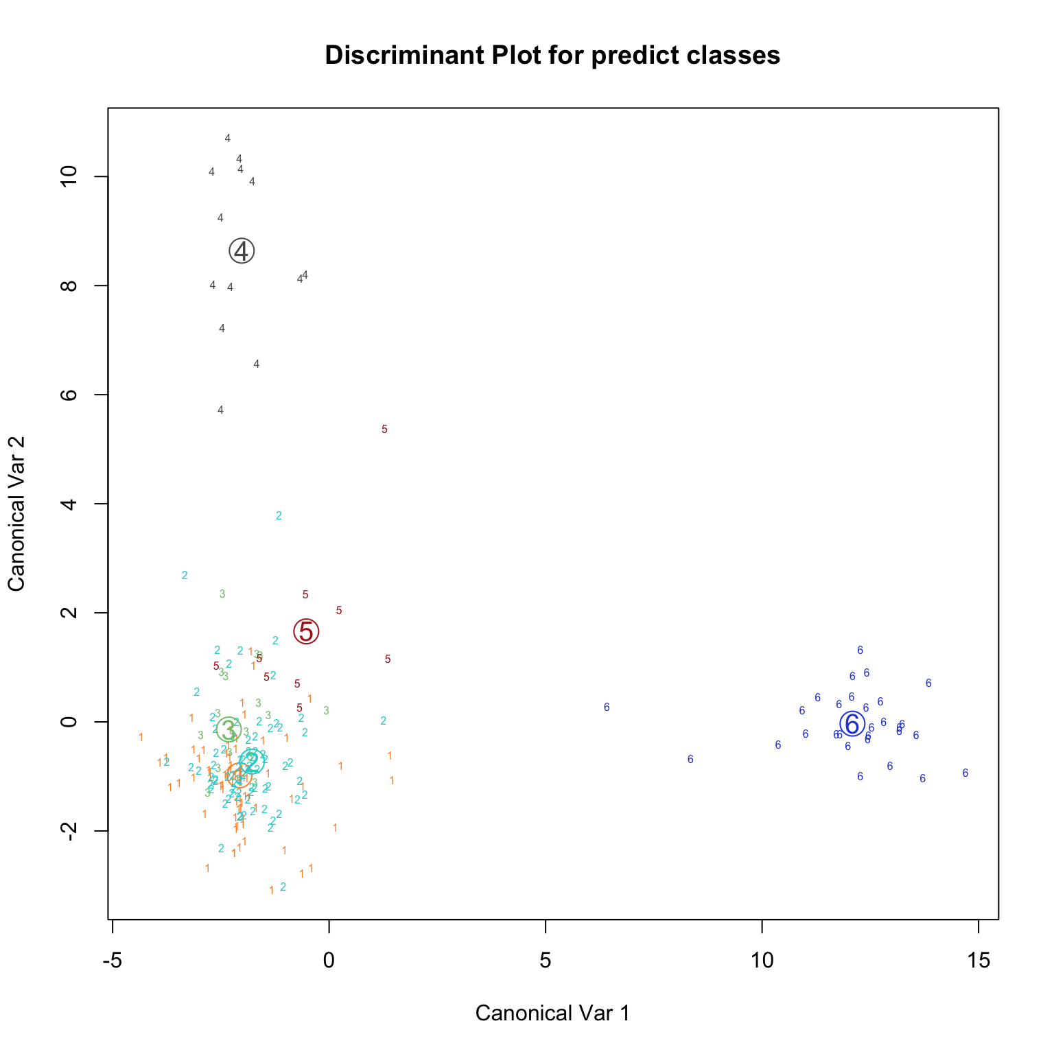
It is clear that all of the action happens along affine subspace \(L \subset \mathbb{R}^p\) of dimension at most \((K-1)\).
Suggests we can / should reduce dimension …
Given a data matrix \({X}_{n \times p}\) and labels \(L \in \{1,\dots,K\}^n\) consider a linear combination \(Xv\)
The SSE of \(Xv\) can be decomposed as
\[ \begin{aligned} v'\widehat{\Sigma}_T v &= \frac{1}{n}\sum_{i=1}^n ((Xv)_i - \overline{Xv})^2 \\ &= \frac{1}{n} \biggl(\sum_{k=1}^K n_k (\overline{Xv}_k - \overline{Xv})^2 \\ & \qquad \quad + \frac{1}{n} \sum_{k=1}^K \sum_{j:L_i=k} ((Xv)_{j} - \overline{Xv}_k)^2 \biggr)\\ &\overset{def}{=} v'\widehat{\Sigma}_B v + v'\widehat{\Sigma}_Wv \end{aligned} \]
Directions \(v\) with high between variance should be important for classification.
Candidate for a good direction
\[ \widehat{v} = \text{argmax}_{v: v'\widehat{\Sigma}_Wv = 1} v'\widehat{\Sigma}_Bv \]
i.e. maximize between groups variance subject to within group variance of 1.
\[ \widehat{\Sigma}_B v = \lambda \widehat{\Sigma}_W v \]
Can construct up to \(K-1\) different directions (subject \(\widehat{v}_i'\widehat{\Sigma}_W \widehat{v}_j = \delta_{ij}\)).
Define the Fisher discriminant scores
\[ V_j = X \widehat{v}_j, 1 \leq j \leq K-1 \]
iris\[ \bar{V}_i = \text{mean of ${V}$ in class $i$}. \]

Source: Wikipedia
\[ Y_{il} = 1_{\{L_l=i\}}, 1 \leq l \leq n, 1 \leq i \leq K-1 \]
We can put the data matrices \({Y}, {X}\) through CCA yielding \(K-1\) pairs \((\widehat{a}_i, \widehat{b}_i), 1 \leq i \leq K-1\) of canonical directions.
It turns out that \(\widehat{b}_i = \widehat{v}_i\) (up to a scalar multiple)…
\[ \lambda \hat{\Sigma}_Tv = \hat{\Sigma}_B v \iff \lambda (\hat{\Sigma}_B + \hat{\Sigma}_W)v = \hat{\Sigma}_B v \]
\[ \lambda \hat{\Sigma}_Wv = \hat{\Sigma}_B v \]
Suppose some of the \(\mu_i\)’s are collinear \[ \text{dim}(L) < K-1 \]
Then, some of the Fisher scores will have little information.
We can discard some of the scores and then classify according to the nearest centroid of reduced space.
Really, to classify, we just need good centroids and some covariance for use in Mahalanobis distance.
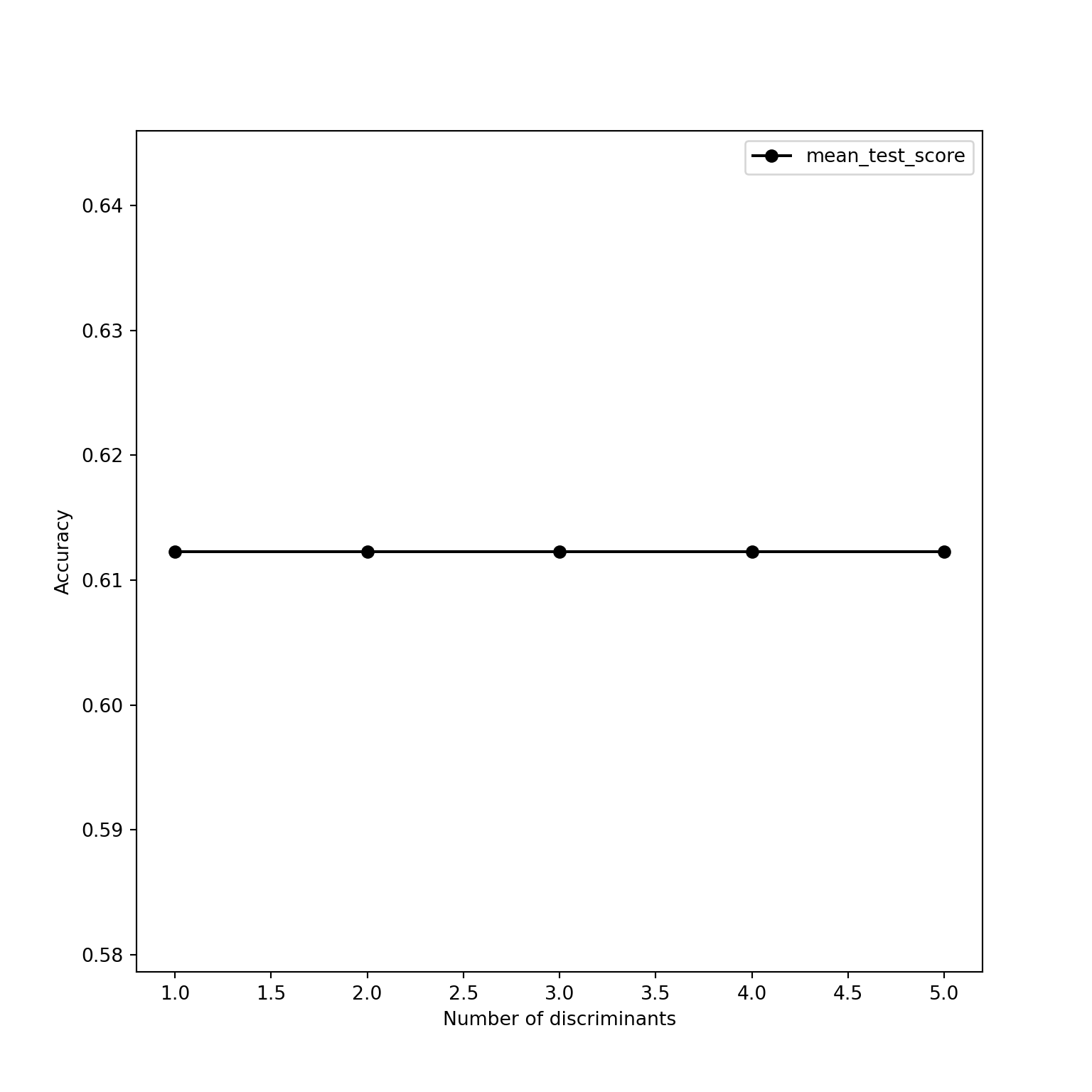
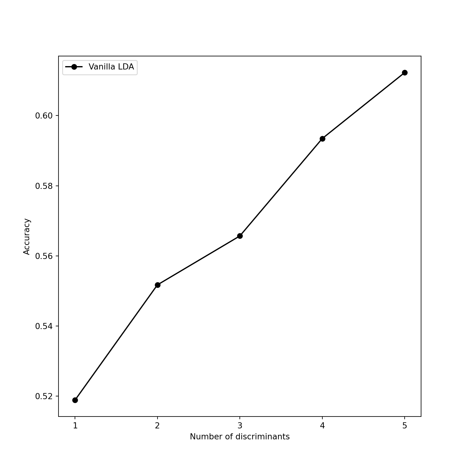
n_components?sklearn ignores n_components in fit and predict… see documentationLDA as a transformUsual generalizations apply:
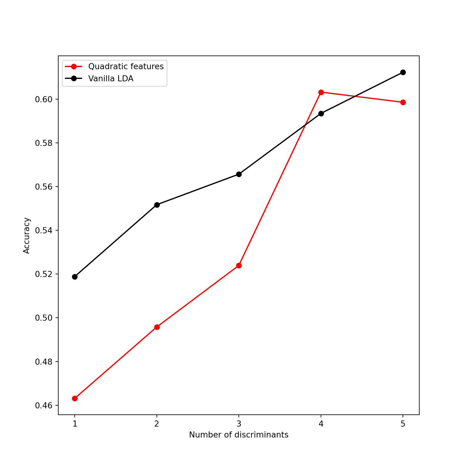
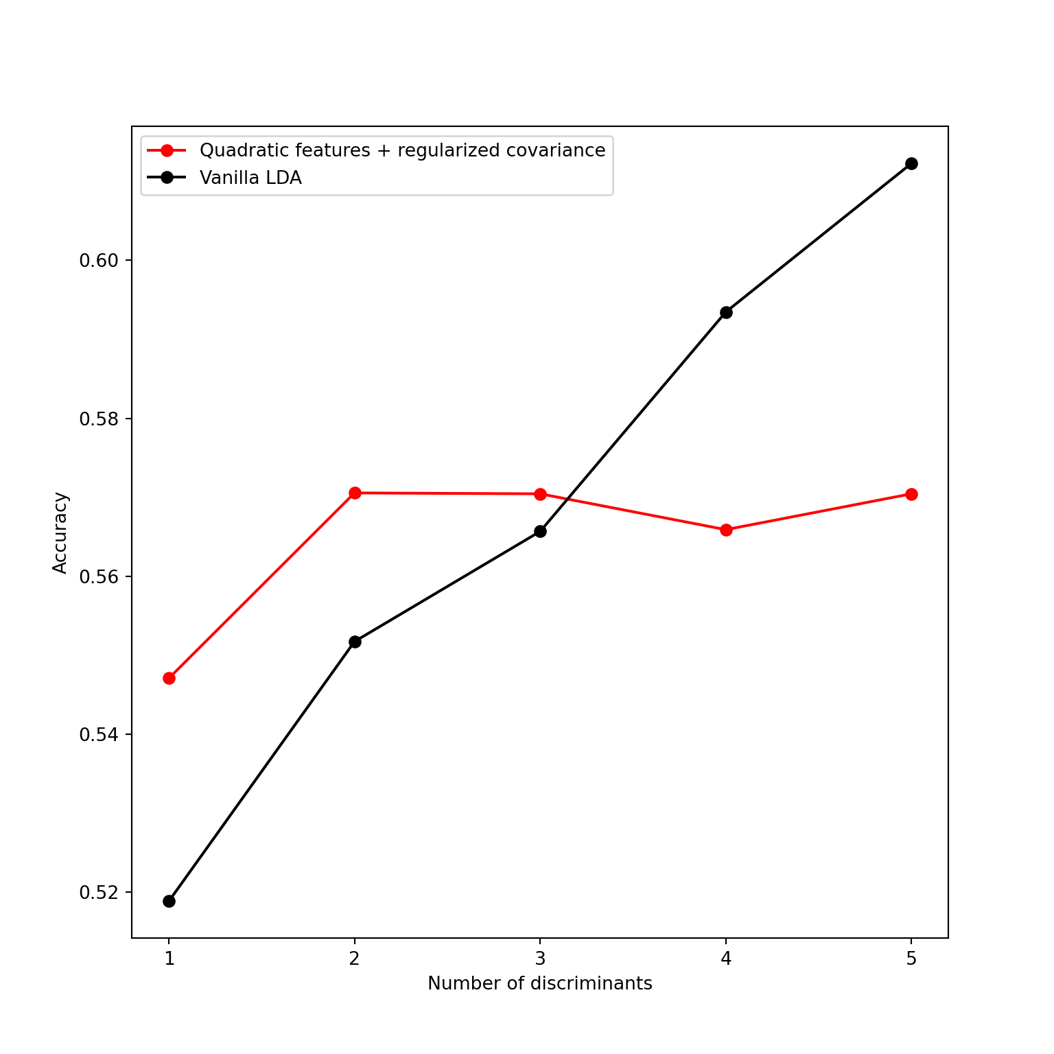
create new features
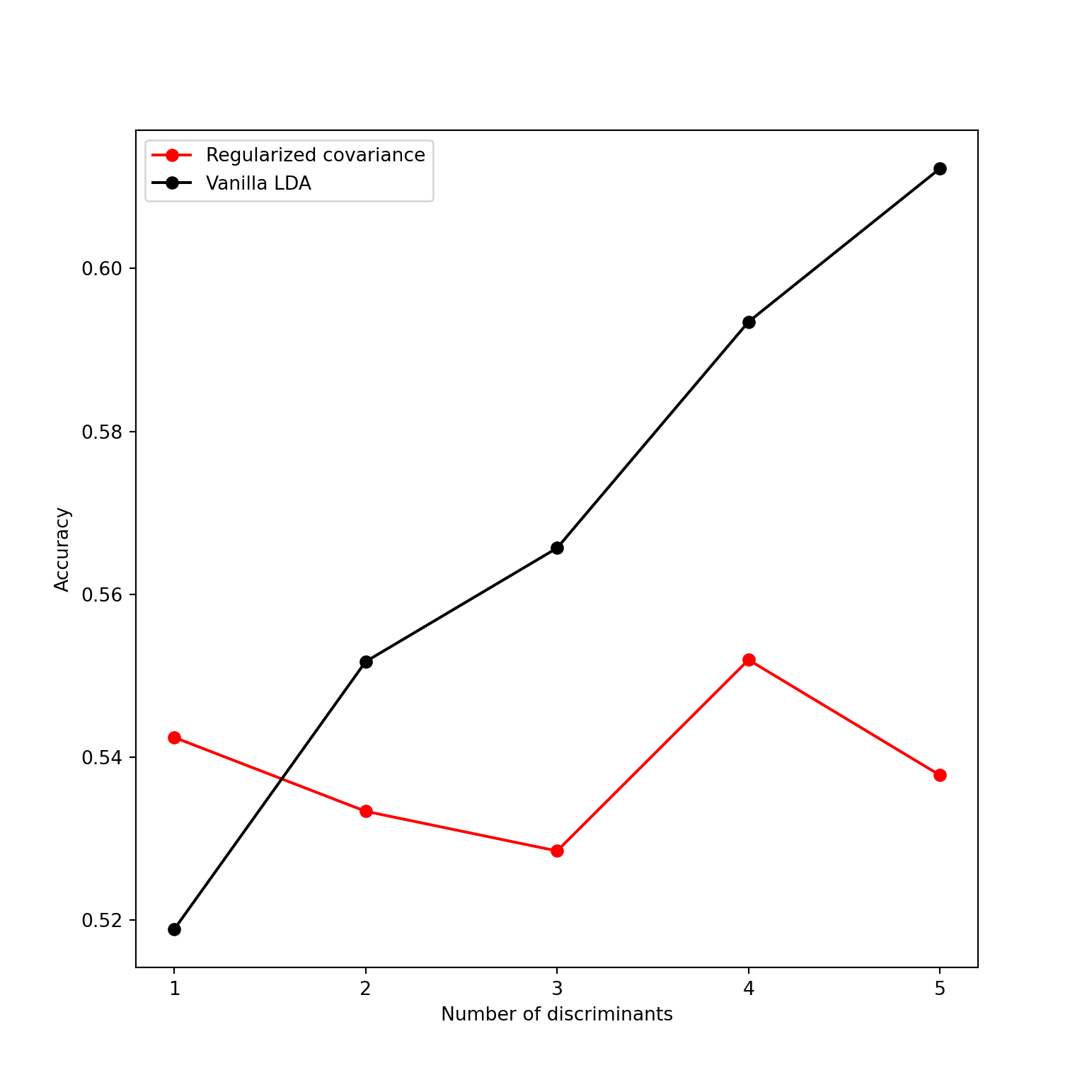
regularize covariance estimates
impose structure on discriminant functions
If we transform \(X \in \mathbb{R}^p\) to \(f(X) \in \mathbb{R}^q\), LDA on \(f(X)\) will produce boundaries that are linear in the components of \(f(X)\).
For example, suppose \(p=2\), take \(f(x)=(x_1, x_2, x_1^2, x_2^2, x_1x_2)\).
This will produce discriminant functions \[ f_{ij}(x) = a_{ij,1} x_1 + a_{ij,2} x_2 + a_{ij,3} x_1^2 + a_{ij,4} x_2^2 + a_{ij,5} x_1 x_1 + c_{ij} \]
Cheap way to get quadratic boundaries, not exactly QDA.
         true
predicted  1  2  3  5  6  7
        1 53 15  3  0  0  0
        2 14 60  2  0  0  0
        3  3  1 12  0  0  0
        5  0  0  0 13  0  0
        6  0  0  0  0  9  0
7 0 0 0 0 0 29sklearnWhy limit ourselves to quadratic?
We could take a large basis \(f(x)=(f_1(x), \dots, f_m(x))\) and perform LDA on \(f({X})\) with labels \(L\).
If we take all \(K-1\) fisher scores, the number of coefficients we need to estimate is \((K-1) * m\) – this grows quickly.
We may also have to invert large matrices… regularize?
LDA / Fisher’s method presumes that a single centroid (and common spread) is sufficient to describe a class.
Within class densities are \(N(\mu_j,\Sigma)\)…
A richer model could use a mixture for within class density:
\[ F_j = \sum_{l=1}^{n_j} \pi_{jl} N(\mu_{jl}, \Sigma_{jl}) \]
Or use common \(\Sigma_{jl}=\Sigma\)…
Can run EM within each class to fit a mixture. Given the mixture, the Bayes or ML rule is easy…
ESL describes this as a compromise between LDA and nearest-neighbor classifier.
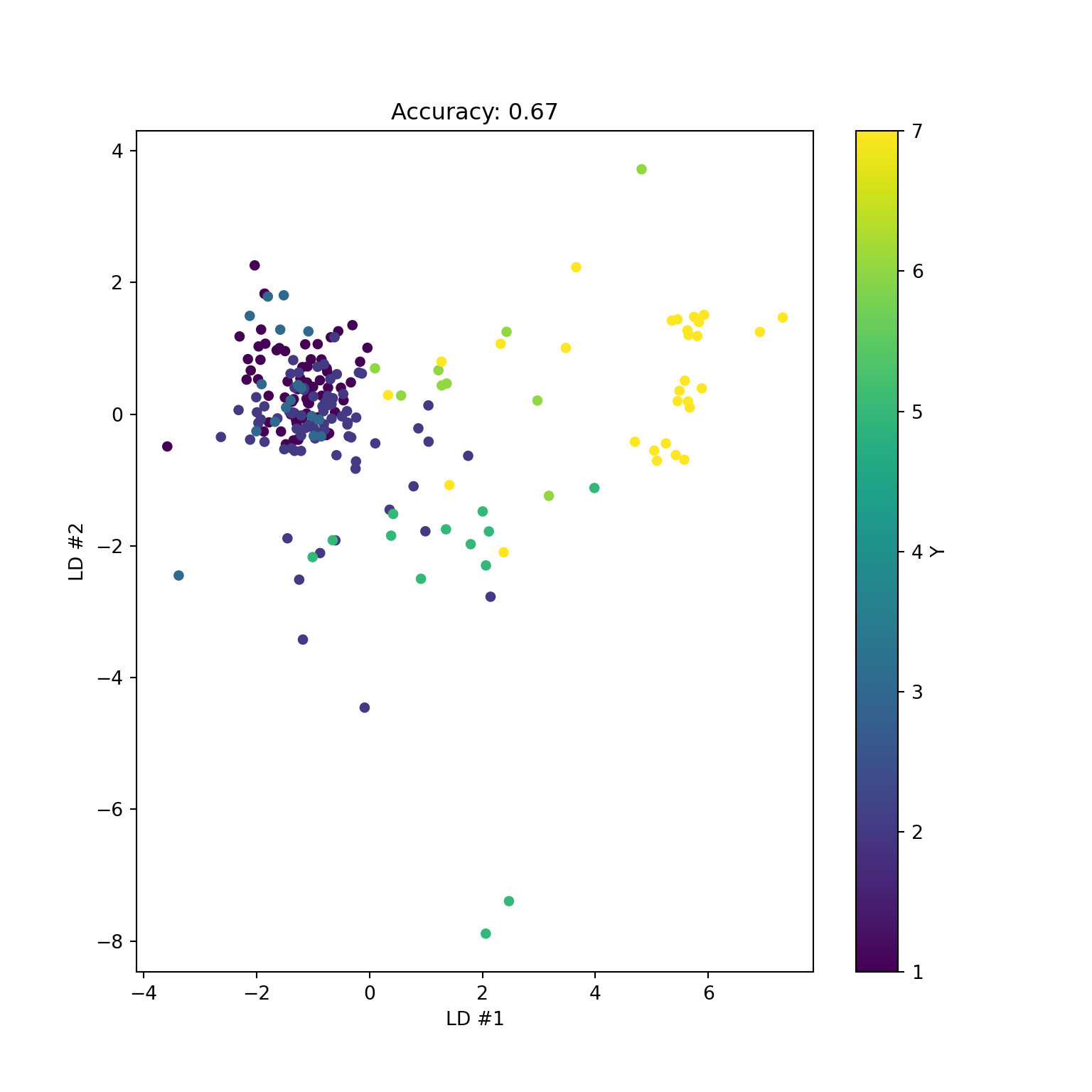
glass.lda = mda::fda(Type ~ ., data=glass)
glass.mda = mda::mda(Type ~ ., data=glass, subclasses=3)
glass.mda
Call:
mda::mda(formula = Type ~ ., data = glass, subclasses = 3)
Dimension: 9
Percent Between-Group Variance Explained:
v1 v2 v3 v4 v5 v6 v7 v8 v9
72.22 84.08 91.74 96.57 98.19 99.13 99.53 99.82 100.00
Degrees of Freedom (per dimension): 10
Training Misclassification Error: 0.23832 ( N = 214 )
Deviance: 323.574 [1] 0.7616822[1] 0.6728972Call:
mda(formula = Type ~ ., data = glass, subclasses = 3, dimension = 4)
Dimension: 4
Percent Between-Group Variance Explained:
v1 v2 v3 v4
61.29 82.85 91.80 96.44
Degrees of Freedom (per dimension): 10
Training Misclassification Error: 0.27103 ( N = 214 )
Deviance: 349.506 [1] 0.728972As in CCA, we must implicitly invert \(\hat{\Sigma}_W\) to compute Fisher’s score (or to fit LDA).
We can simplify the model by assuming that \(\Sigma_j\) is diagonal in QDA – this leads to Naive Bayes
\[ f(X|Y=l) = \prod_{j=1}^p f_{j}(X_j|Y=l) \]
\[ f_j(x|Y=l) = N(\mu_j, \sigma^2_j) \]
Assuming a diagonal covariance is form of regularization on the covariance…
ESL also defines Diagonal LDA – use common diagonal covariance.
\[ \widehat{\Sigma}_j(\gamma) = \gamma \widehat{\Sigma}_j + (1 - \gamma) \widehat{\Sigma}_{\text{pooled}} \]
or
\[ \widehat{\Sigma}_j(\gamma) = \gamma \widehat{\Sigma}_j + (1 - \gamma) \widehat{\sigma}^2 I \]
One can also regularize the centroid estimates.
Neareast Shrunken Centroids combines diagonal LDA with regularization.
For each feature \(l\), soft-threshold \(\bar{X}_{j,l} - \bar{X}_l\) (or more precisely the \(Z\)-scores).
Forces many features to share common centroid value \(\hat{\mu}_{j,l}\) – means they effectively do not contribute to classification rule
\[ x \mapsto \text{argmin}_l \frac{1}{2} \sum_{j=1}^p \frac{ \left(x_j - \hat{\mu}^{\lambda}_{j,l}\right)^2 }{ \widehat{\sigma}^2_j} - \log \pi_l \]

(Source: ESL)