Factor analysis
\[
\Sigma = \sigma^2 I + V V^T
\]
More generally, we could assume
\[
\Sigma = \Psi + \Gamma \Gamma^T, \qquad \Gamma \in \mathbb{R}^{p \times k}
\]
and \(\Psi\) a diagonal matrix. (Book uses \(\Lambda\) for my \(\Gamma\) ).
Probabilistic PCA vs Factor Analysis
Suppose \(A=\text{diag}(a_1, \dots, a_p)\) then \[
AX \sim N\left(A\mu, A^2 \Psi + A \Gamma \Gamma^TA^T\right)
\]
\(\implies\) a factor model remains a factor model
\(\implies\) not true for PPCA!
If \(R\) is an orthogonal rotation then
\[
RX \sim N\left(R\mu, RVV'R' + \sigma^2 I\right)
\]
\(\implies\) PPCA model is preserved but factor model is not…
Likelihood of factor analysis model
In the normal model, there is a well-defined likelihood (with \(R_c\) we’ve profiled out \(\mu\) ..)
\[
\ell(\Gamma,\Psi|X) = \frac{n}{2} \log \det(2\pi(\Psi + \Gamma \Gamma^T)) + \frac{1}{2} \text{Tr}((\Psi + \Gamma \Gamma^T)^{-1}X^TR_cX)
\]
(Negative-log)-likelihood not really amenable to simple algorithms to minimize over \((\Psi,\Gamma)\) .
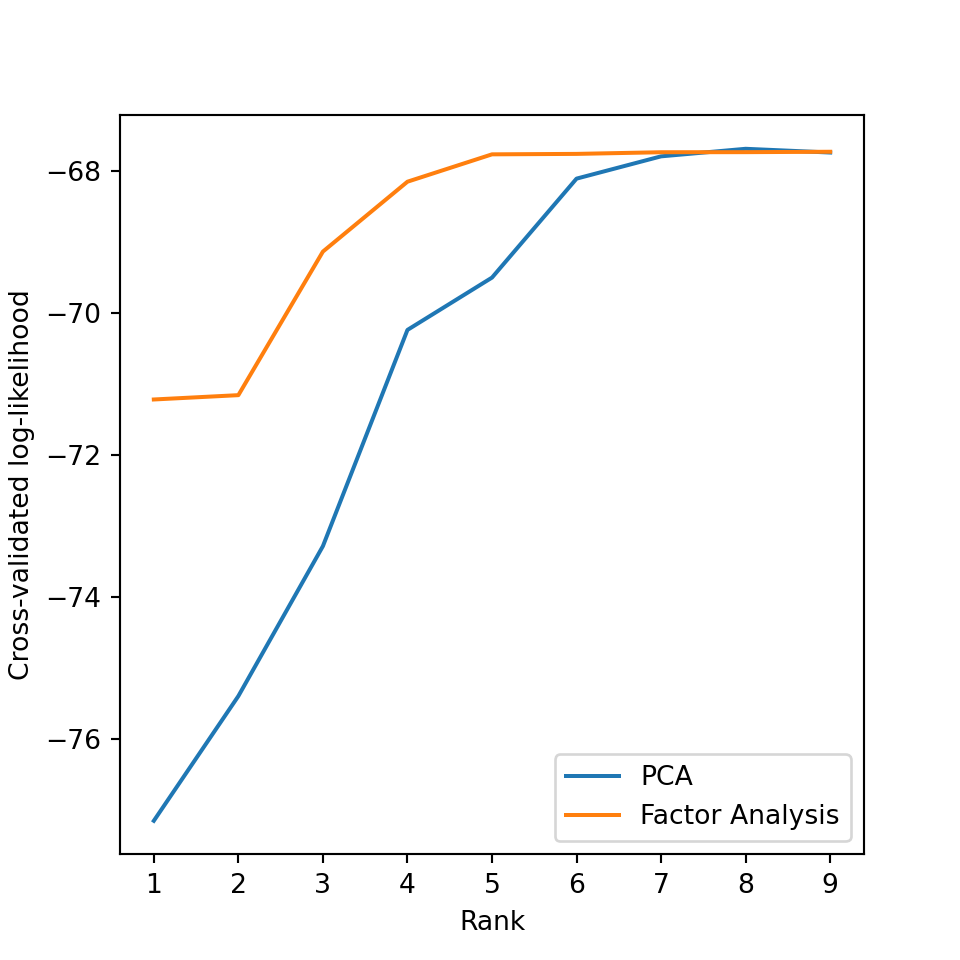
Still, having a log-likelihood opens up AIC / BIC / CV for choosing rank \(k\) .
Generative model
Similar to Probabilistic PCA:
\[
\begin{aligned}
Z & \sim N(0, I_{q \times q}) \\
X|Z &\sim N(VZ, \Psi)
\end{aligned}
\]
Estimation of factor analysis model
In the population setting, note that if \(\Psi\) is known
\[
\Sigma - \Psi = \Gamma \Gamma^T = V \Lambda V^T
\]
Hence, we might take \(\Gamma = V[,1:k]
\Lambda[1:k]^{1/2}\) , based on leading rank \(k\) eigendecomposition of \(\Sigma-\Psi\) .
Principal factor analysis for rank \(k\)
Start with initial estimate \(\widehat{\Psi}^{(1)}\) and covariance (or correlation) matrix \(\widehat{\Sigma}\) .
For \(i=1,\dots\) , run rank \(k\) eigendecomposition on \(\widehat{\Sigma}-\widehat{\Psi}^{(i)}\) yielding
\[
\widehat{\Gamma}^{(i)} = V^{(i)}[,1:k] D^{(i)\, {1/2}}[1:k]
\]
\[
\widehat{\Psi}^{(i+1)} = \text{diag}\left(\widehat{\Sigma} - \widehat{\Gamma}^{(i)} \widehat{\Gamma}^{(i)\, T} \right)
\]
Factor analysis for flow data (MLE)
 [1] "converged"    "loadings"     "uniquenesses" "correlation"  "criteria"
 [6] "factors"      "dof"          "method"       "rotmat"       "scores"
[11] "STATISTIC"    "PVAL"         "n.obs"        "call"
Call:
factanal(x = flow, factors = 2, scores = "regression")

Uniquenesses:
   V1    V2    V3    V4    V5    V6    V7    V8    V9   V10   V11
0.014 0.005 0.816 0.841 0.998 0.979 0.786 0.955 0.038 0.046 0.315

Loadings:
    Factor1 Factor2
V1   0.121   0.986
V2   0.148   0.987
V3   0.371   0.215
V4   0.352   0.189
V5
V6   0.145
V7   0.389   0.249
V8  -0.164  -0.136
V9   0.978
V10  0.971   0.102
V11  0.822

               Factor1 Factor2
SS loadings      3.072   2.133
Proportion Var   0.279   0.194
Cumulative Var   0.279   0.473

Test of the hypothesis that 2 factors are sufficient.
The chi square statistic is 22471.07 on 34 degrees of freedom.
The p-value is 0
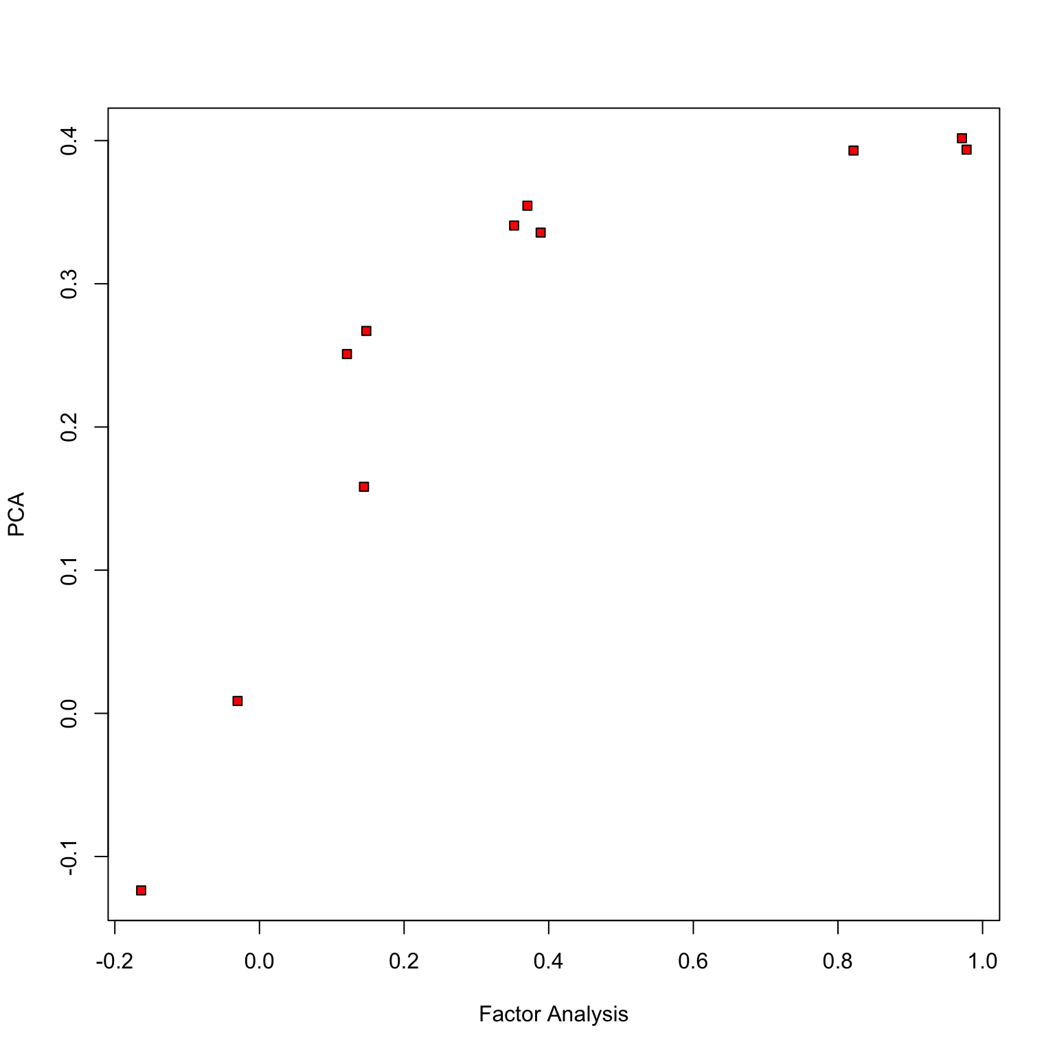
Compare to PCA (1st loading)
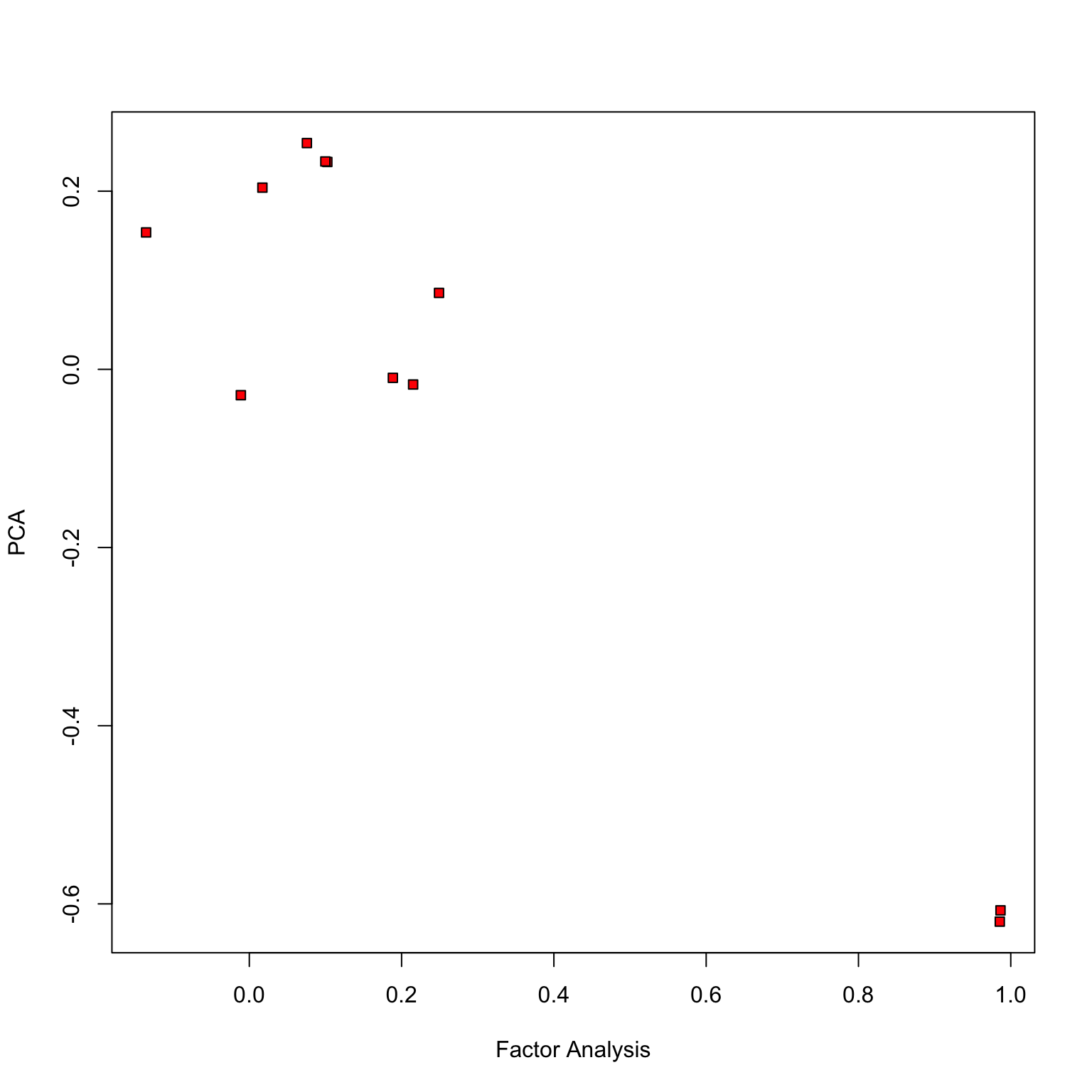
Compare to PCA (2nd loading)
Latent scores
Scores \(Z\) are such that
\[
X|Z \sim N(\Gamma Z, \Psi)
\]
suggesting that, given an estimate \((\Gamma, \Psi)\) we can recover \(Z\) from \(X\) by regression (Bartlett’s scores )
\[
\widehat{Z} = (\Gamma^T\Psi^{-1}\Gamma)^{-1} \Gamma^T\Psi^{-1}X
\]
Alternatively (Thomson’s scores )
\[
E[Z|X] = (I+\Gamma^T\Psi^{-1}\Gamma)^{-1}\Gamma^T\Psi^{-1}X
\]
Thomson has lower MSE, Bartlett’s is unbiased…
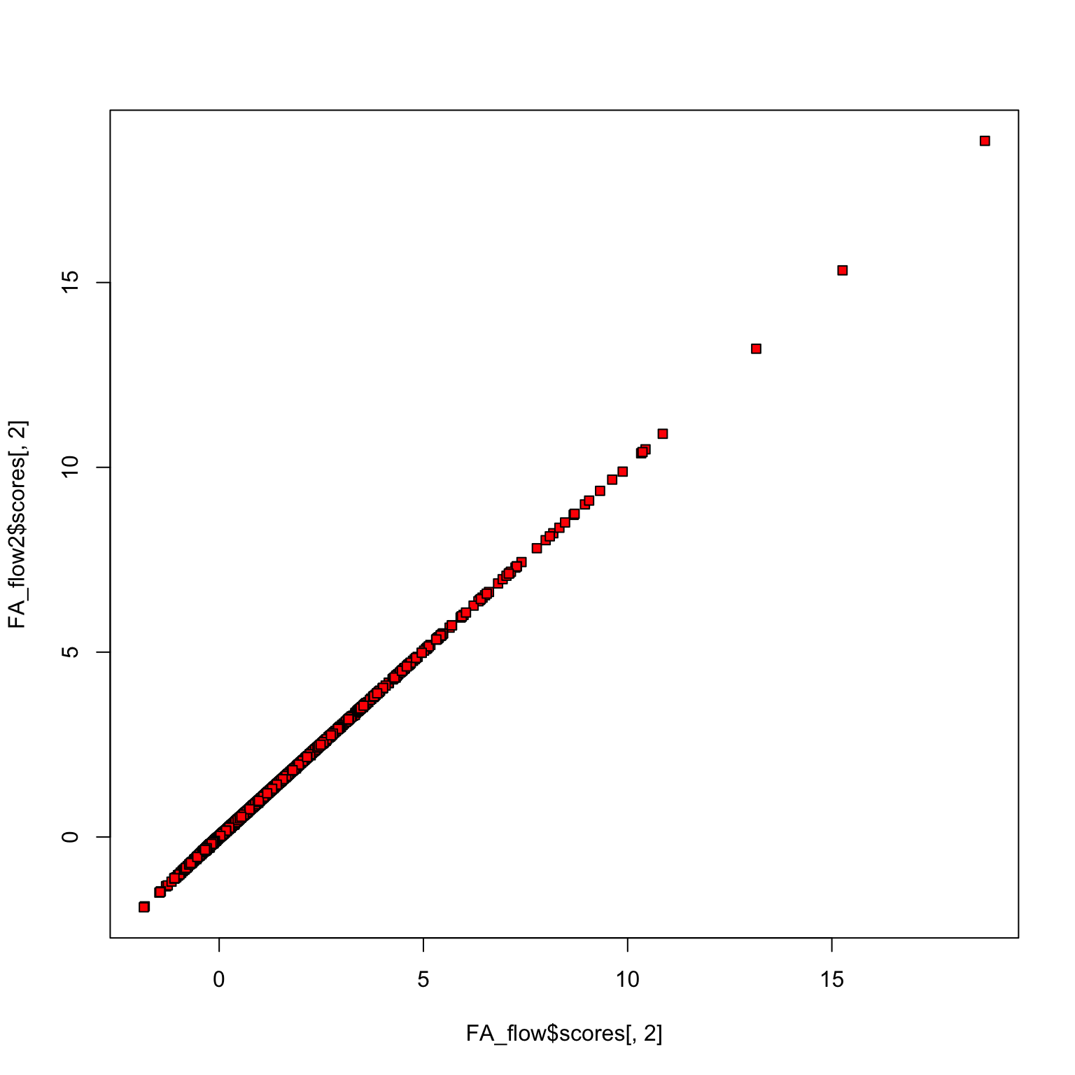
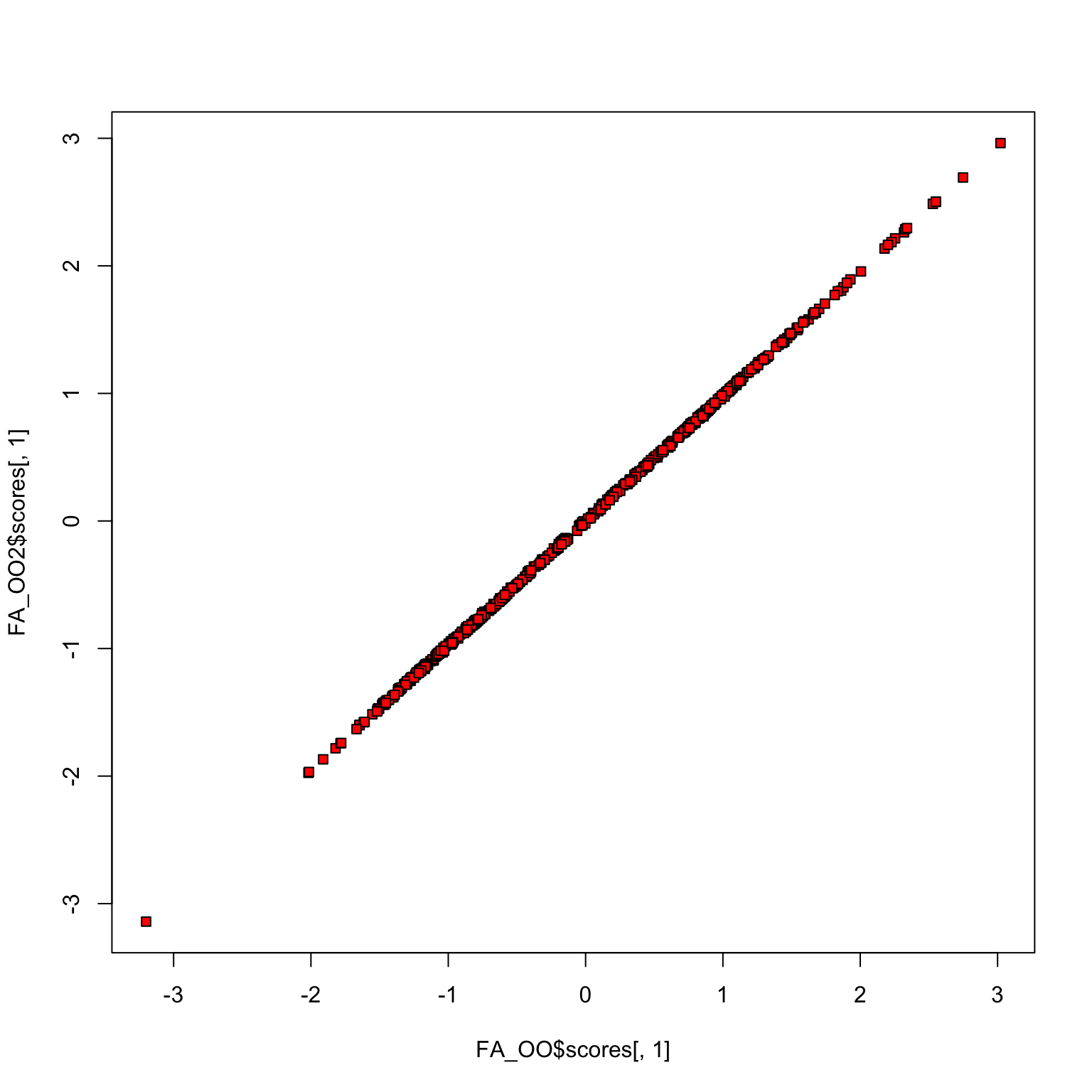
Comparing scores
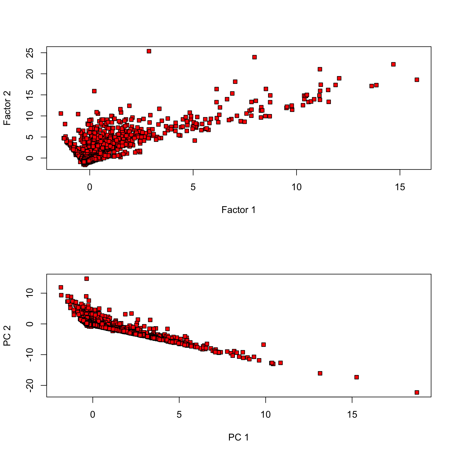
Comparing Thomson vs. Bartlett scores
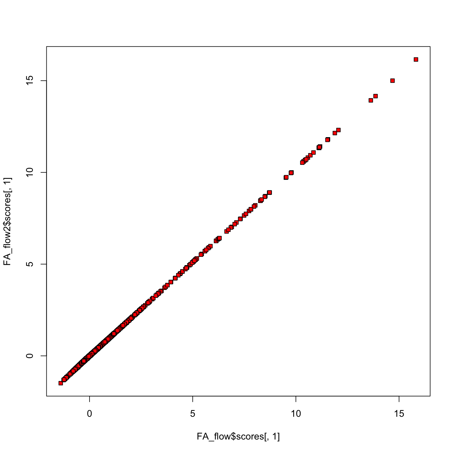
Comparing Thomson vs. Bartlett scores
Olive oil data
library (pdfCluster)data (oliveoil)= oliveoil[,3 : 10 ]= factanal (OO, 2 , scores= 'Bartlett' )= factanal (OO, 2 , scores= 'regression' )
How many factors can we fit?
Remaining degrees of freedom after we fit for \(k\) factors is
\[
1/2(p-k)^2 - 1/2(p+k)
\]
MLE can still be challenging for factanal
= 3 ; p = 11 print (0.5 * ((p - k)^ 2 - (p + k)))tryCatch ({<- factanal (flow, k)error = function (e) {paste ("Factanal failed with k =" , k, ". Error:" , e$ message)
[1] "Factanal failed with k = 3 . Error: unable to optimize from this starting value"
Latent variables and EM
Likelihood is somewhat hard to maximize having observed only \(X\) .
BUT, if we observed \(Z\) , estimation is easy…
Estimation of \(\Gamma\) would be a multivariate regression of \(X\) onto \(Z\) .
Estimation of \(\Psi\) would be easy: take diagonal part of usual MLE of \(\widehat{\Sigma}\) in the above regression.
Suggests EM algorithm is a nice fit for factor analysis…
EM for factor analysis
Complete (negative) log-likelihood
\[
\frac{n}{2} \log \det \Psi + \frac{1}{2} \left[\text{Tr}\left(\Psi^{-1} (X-ZV')'(X-ZV')\right) + \frac{1}{2} \|Z\|^2_F \right]
\]
Note that \(Z|X \sim N\left(V'(VV' + \Psi)^{-1} X, I - V'(VV' + \Psi)^{-1}V\right)\)
Expected value given \(X\) at \((V_{\text{cur}}, \sigma^2_{\text{cur}}) = (V_c, \sigma^2_c)\) (ignoring irrelevant terms)
\[
\frac{n}{2} \log \det \Psi + \frac{1}{2}\text{Tr}(\Psi^{-1}\left(X'X - 2 X'\mathbb{E}_{V_c,\sigma^2_c}[Z|X]V' + V \mathbb{E}_{V_c,\sigma^2_c}[Z'Z|X]V' \right)
\]
Estimation of new \((V_{\text{new}}, \Psi_{\text{new}})\) : multi response regression with covariance \(I_{n \times n} \otimes (\sigma^2 I_{p \times p})\) …
A convex version of factor analysis?
In the factor analysis model \(\Sigma^{-1}\) also has a particular structure.
For arguments sake, let’s assume \(\Psi=I\) and \(\Gamma^T\Gamma=\kappa I\) . Then,
\[
\Sigma^{-1} = I - \frac{\kappa}{\kappa + 1} \Gamma \Gamma^T
\]
Let \(\Theta = \Sigma^{-1} = \Phi - \Gamma \Gamma^T = \Phi - \Omega\) :
\[
\ell(\Phi,\Omega|X) = - \frac{n}{2} \log \det(\Phi - \Omega) + \text{Tr}(X^TR_cX(\Phi - \Omega))
\]
subject to \(\Phi\) being diagonal and \(\Omega\) is rank \(k\) (implicitly \(\Phi - \Omega > 0\) )
Convex relaxation
The rank constraint is not convex but the usual surrogate for rank is nuclear norm
\[
\text{minimize}_{(\Phi, \Omega)} = - \frac{n}{2} \log \det(\Phi - \Omega) + \text{Tr}(X^TR_cX(\Phi - \Omega)) + \lambda \|\Omega\|_*
\]
\[
\text{minimize}_{(\Phi, \Omega): \Phi-\Omega \geq 0, \Omega \geq 0} = - \frac{n}{2} \log \det(\Phi - \Omega) + \text{Tr}(X^TR_cX(\Phi - \Omega)) + \lambda \|\Omega\|_*
\]
subject to \(\Phi\) being diagonal.
Similar model considered in Chandrasekaran et al. – relaxed diagonal \(\Phi\) to sparse \(\Phi\) . Combination of factor analysis and graphical LASSO.
Fitting with sklearn
= FactorAnalysis(n_components= 3 )
FactorAnalysis(n_components=3) In a Jupyter environment, please rerun this cell to show the HTML representation or trust the notebook.
array([ -63.97497457,  -63.76032192,  -63.62579767, ...,  -63.71528559,
       -102.21877799,  -63.70396606])
= PCA(n_components= 3 )
PCA(n_components=3) In a Jupyter environment, please rerun this cell to show the HTML representation or trust the notebook.
# uses PPCA likelihood
array([-68.11612015, -68.13057038, -68.09813484, ..., -67.90037491,
       -85.06534907, -68.09755384])