Multidimensional scaling
Multidimensional scaling

A popular visualization technique
Observation: a distance / dissimilarity matrix \[ D_{ij} \overset{?}{=} d(X_i, X_j) \]
Note: need not be a distance but we usually assume
\[ D_{ij} \geq 0, D_{ii}=0 \]
Goals of MDS
Learn something about structure of the sample.
In MDS learn something means find a \(k\)-dimensional Euclidean representation \(\hat{X} \in \mathbb{R}^{n \times k}\)
We’ll call this a visualization – MKB calls it a configuration.
PCA and MDS
- Recall what we hope to find with rank \(k\)- PCA
\[ X \overset{D}{=} \mu + \sum_{j=1}^k \langle V_j, (X - \mu) \rangle \cdot V_j + \text{small error} \]
By taking only the first \(k\) principal components we get an optimal \(k\)-dimensional Euclidean representation.
Let \(\hat{X}_k\) be the rank \(k\) SVD of (centered) \(X\), then
\[ \hat{X}_k = U_k \Lambda_k V_k^T = \text{argmin}_{Y:\text{rank}(Y)=k} \frac{1}{2} \|X-Y\|^2_F \]
Consider the \(n \times n\) similarity matrix \(S=RXX^TR\), with \(R\) the centering matrix \(I-\frac{1}{n}11^T\).
Its rank \(k\)-approximation is
\[ U_k \Lambda_k^2 U_k^T \]
This is the similarity matrix of the best rank \(k\) projection of the centered data.
Rank \(k\) decomposition of similarity \(\to\) visualizations that (approximately) preserve distances.
If distances are Euclidean (or close?) then rank \(k\) decomposition of similarity yields optimal \(\hat{X}\).
Euclidean distance matrices
- We say that an distance matrix \(D_{n \times n}\) is Euclidean of dimension \(p\) if there exists a collection of points \(Y \in \mathbb{R}^{n \times p}\) such that
\[ D_{ij} = \|Y[i] - Y[j]\|_{2}\]
- From a Gram matrix \(K\) we can form a distance matrix
\[ D_{ij} = (K_{ii} - 2 K_{ij} + K_{jj})^{1/2} \]
Gram matrices are Euclidean
Fact: any Gram distance matrix is Euclidean with \(p=\text{rank}(K)\).
Write \(K=U\Lambda^2U^T\) and take \(\hat{X}=U\Lambda\) from which we see
\[ K_{ij} = \hat{X}[i]^T\hat{X}[j] \]
and
\[ D_{ij} = \|\hat{X}[i]-\hat{X}[j]\|_2 \]
For Euclidean distance matrices, taking \(k=p\) and setting \(\hat{X} \in \mathbb{R}^{p \times n}\) we perfectly reconstruct distances \((D_{ij})_{1 \leq i,j \leq n}\).
Projecting \(\hat{X} \in \mathbb{R}^p\) to lower-dimensional space might kill some noise (and make it easier to see structure).
Classical MDS solution
Not all distance matrices are Euclidean… but we can try.
Given a distance matrix \(D\), define
\[ \begin{aligned} A_{ij} &= -\frac{1}{2} D_{ij}^2 \\ \end{aligned} \]
and
\[ B = RAR \]
- Note that if \(D\) were formed from a centered data matrix
\[ D_{ij}^2 = \|RX[i] - RX[j]\|^2_2 = (RXX^TR)_{ii} - (2RXX^TR)_{ij} + (RXX^TR)_{jj} \]
so
\[ A = -s1^T-1s^T + RXX^TR \]
with \(s = \text{diag}(RXX^TR)/2\) and
\[ B = RXX^TR \]
General case
\(B=B(D)\) is symmetric so it has eigendecomposition \(U \Gamma U^T\).
If the first \(k\) eigenvalues of \(B\) are non-negative, then we take
\[\hat{X}_k(D) = U_k \Gamma_k^{1/2} \in \mathbb{R}^{n \times k}\]
as the rank \(k\) classical MDS solution.
What if we asked for \(k=5\) but only 3 eigenvalues are non-negative? Not completely clear what right thing to do is…
Taking all 5 retains some optimality (c.f. Theorem 14.4.2 of MKB) even though eigendecomposition would not “allow” a 5-dimensional configuration.
Optimality measured by
\[ \mathbb{R}^{n \times n} \ni B \mapsto \text{Tr}(B(D)-B)^2 \]
Classical MDS solution and PCA
In the PCA case, i.e. when \(D\) is formed from a centered data matrix, this is exactly the same as first \(k\) sample principal component scores.
Let’s start with distances from a covariance kernel \(K\):
\[ \begin{aligned} A_{ij} &= -\frac{1}{2} D_{ij}^2 \\ &= K(X_i, X_j) - \frac{1}{2} K(X_i, X_i) - \frac{1}{2} K(X_j, X_j) \end{aligned} \]
– We see that
\[ RAR= RKR \]
Note: this is the same matrix we saw in HW problem on kernel PCA.
In summary: taking leading scores from kernel PCA is classical MDS with distance based on kernel \(K\).
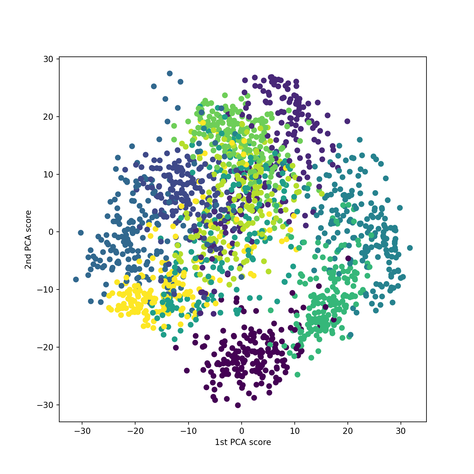
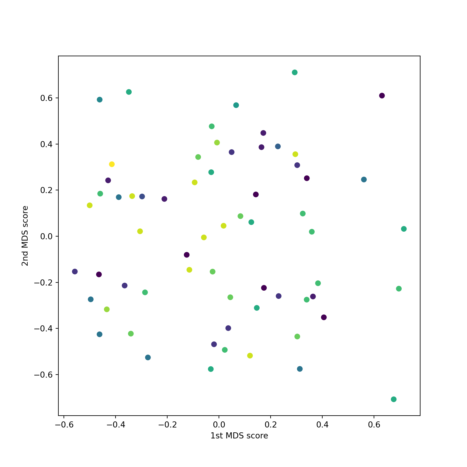
NCI data
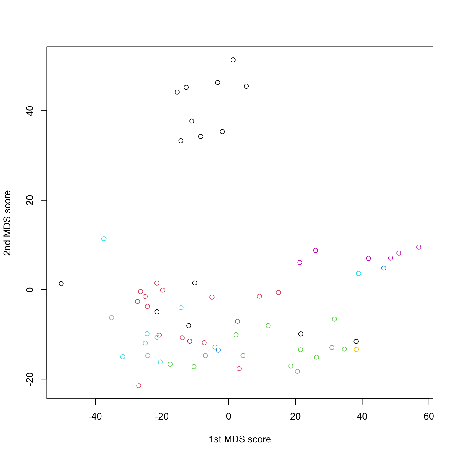
Hmm… R and sklearn don’t agree
Also doesn’t agree with PCA
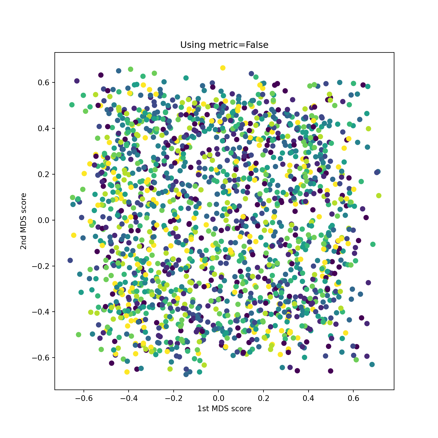
What does sklearn.MDS do?
- Let \(y \in \mathbb{R}^{n \times k}\) denote a visualization with distance matrix
\[ D(y)_{ij} = \|y[i] - y[j]\|_2. \]
- Directly attempts to solve
\[ \text{minimize}_{y_1, \dots, y_n} \sum_{i,j} (D_{ij} - D(y)_{ij})^2 \overset{def}{=} \text{Stress}(y_1, \dots, y_n) \]
- Implements SMACOF algorithm wikipedia, which also allows weights \(w_{ij}\).
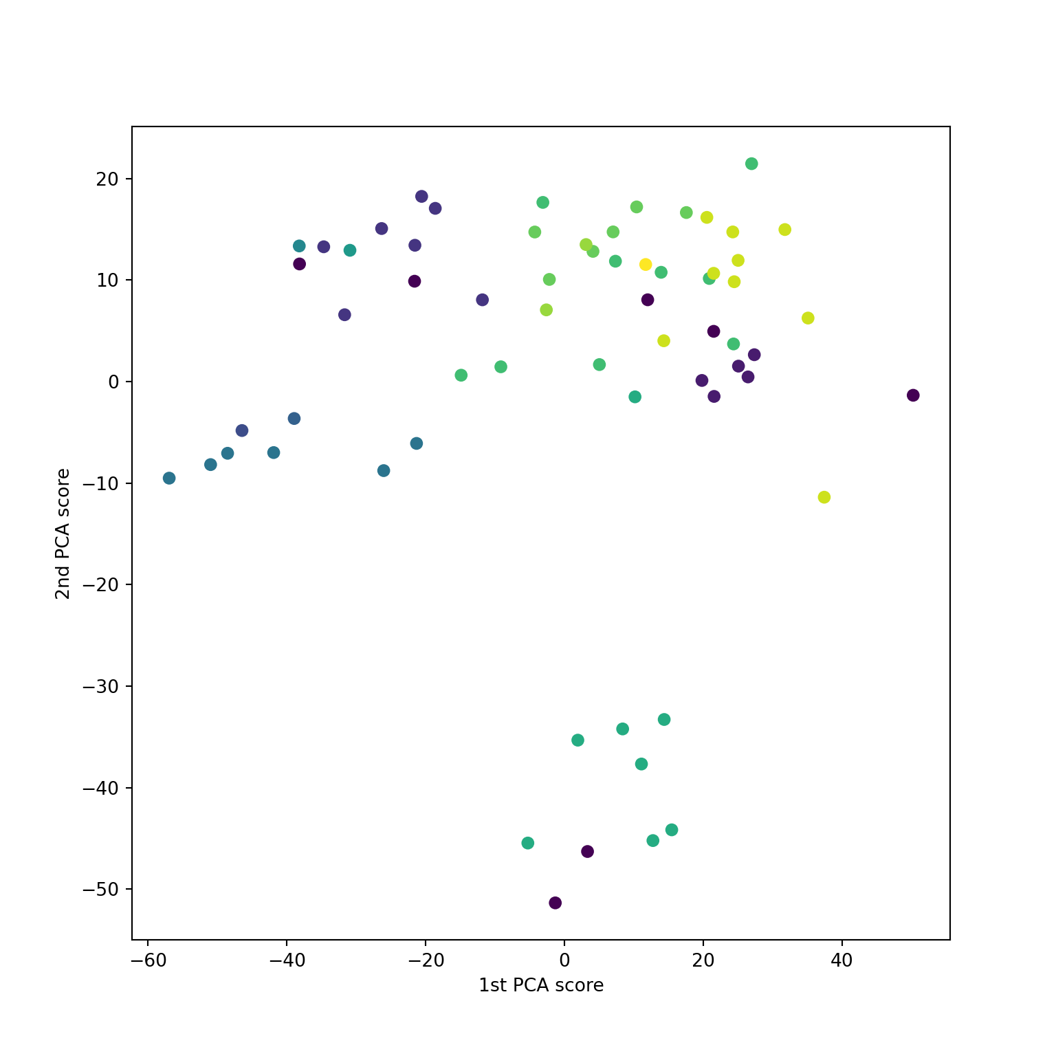
How is classical MDS not just PCA?
MDS methods (usually) work with \(D_{n \times n}\) rather than original features.
As a result, we don’t get loadings / functions on feature space.
Mostly used as visualization technique – not as useful for feature generation / downstream supervised procedures.
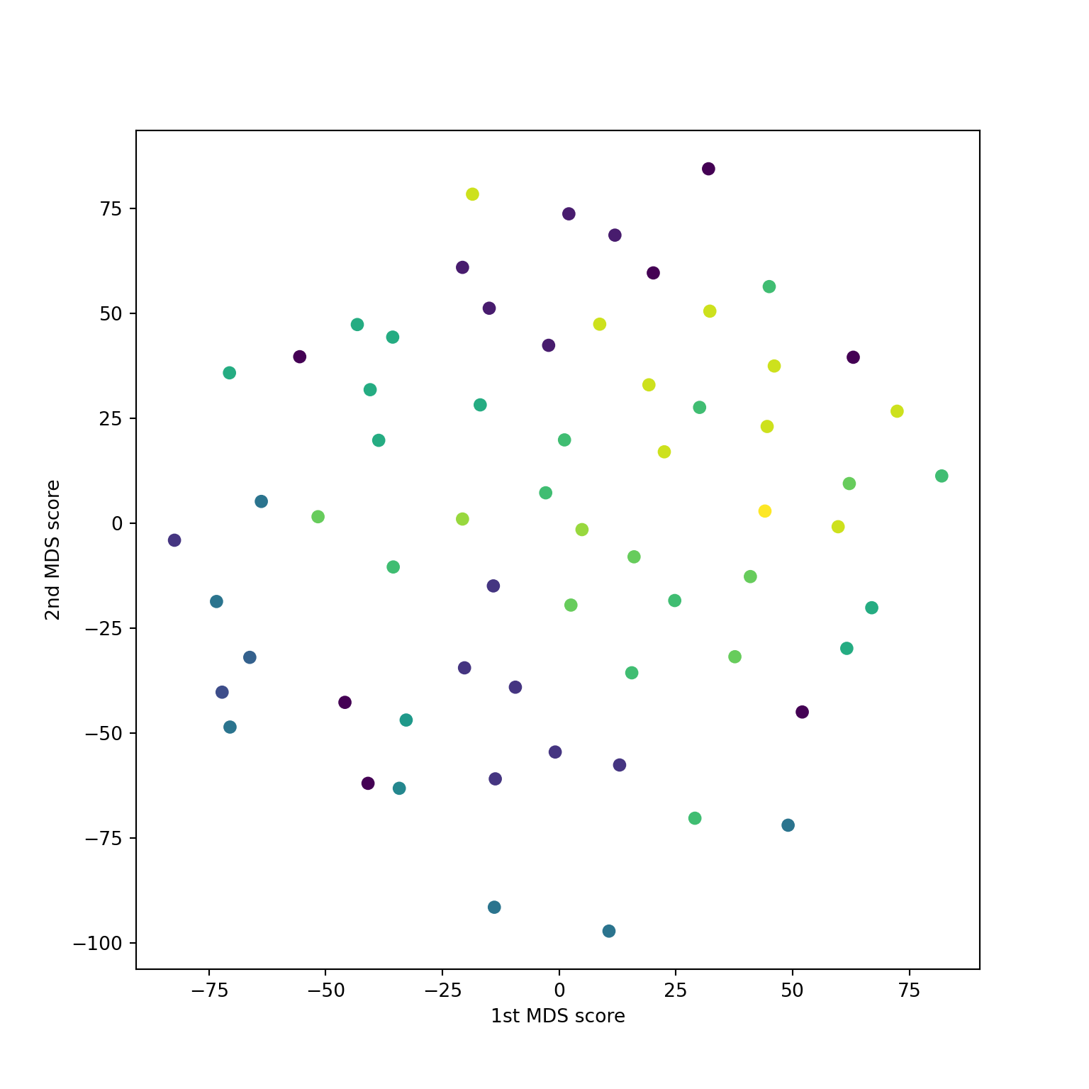
sklearn.MDS on digits
Compare to classical solution
Non-metric solution
Similar inputs to classical case: a distance matrix \(D\) and a dimension \(k\).
Constraint: seeks to have order of pairwise distances preserved in the \(k\)-dimensional approximation / visualization
The non-metric solution tries to impose same ordering on values \(D(Y)\) as \(D\).
- Along with this ordering (isotonic) constraint on \(D(Y)\), it has a cost
\[ \text{Stress}_1(y_1,\dots,y_n) = \sqrt{\frac{ \inf_{D^* \sim D} \sum_{i,j} (D(y)_{ij} - D^*_{ij})^2}{\sum_{i,j} D(y)_{ij}^2}}. \]
- Goal: directly minimize over \((y_1, \dots, y_n)\)
Kruskal algorithm
- At \(k\)-th iteration let’s call configuration \(Y^k\) with distance:
\[ D(y^k)_{ij} = \|y^k[i] - y^k[j]\|_2 \]
Use isotonic regression to find \(\widetilde{D}^k\), the distance matrix satisfying the required ordering that is closest to \(D(y^k)\).
Apply classical solution to \(\widetilde{D}^k\), yielding \(y^{k+1}\).
Repeat 1-3.
Potential problem: \(\widetilde{D}^k\) may be non-Euclidean?
Will terminate when \(Y\) is a configuration respecting the ordering that is \(k\)-Euclidean.
Non-metric for NCI60 data
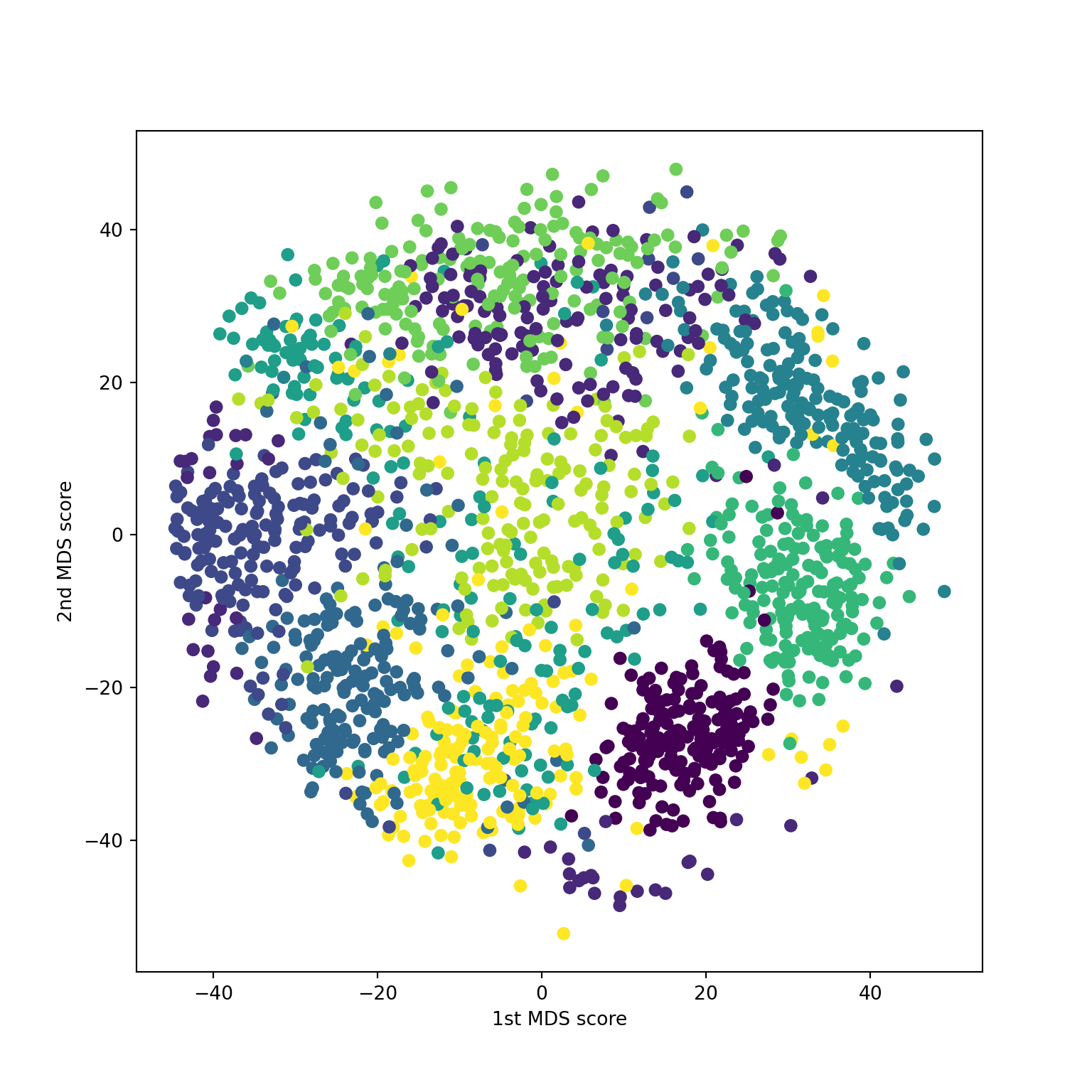
Non-metric on digits data
Variants of MDS
Kruskal’s algorithm directly optimizes over the configuration.
Classical method crosses the fingers and hopes a Euclidean configuration of rank \(k\) exists.
Variants
Graph-based distances
(Essentially) uses classical MDS on distances derived from local properties of the dataset.
E.g. diffusion eigenmaps, ISOMAP
Cost function
Some methods directly optimize over configuration as well with different loss functions.
Local Linear Embedding, t-SNE, local MDS
Manifold learning
MDS looks to find low-dimensional approximation to \(D\), i.e. points in a low dimension \(k\) whose Euclidean distance is close to the distances implied by \(k\).
Essentially a linearization of \(D\)…
Techniques that seek to model more general low-dimensional structure fall under manifold learning umbrella, though many (most?) involve some variant of MDS.
Some examples
ISOMAP
Diffusion / Laplacian maps
Local linear embedding
Graph-based distances
ISOMAP

|

|
- Classical MDS applied to a distance matrix formed by geodesic / graph distance on graph at scale \(r\).
Graph distance
Let \[ D(i,j) = \text{length of shortest path between vertices $i$ and $j$ in $G_k$} \]
We can add weights, too… let \(W=W_{ij}\) be a weight matrix, with \[ W_{ij} = \infty, \ \text{if $i$ not connected to $j$} \]
Set \[ D_W(i,j) = \min_{p: i \mapsto j}\sum_{e \in p} W_{e} \] where \(p\) are all paths to connect \(i\) to \(j\) and a path is described by the edges \(e\) it crosses.

Source: Balasubramanian et al.
LHS: points in curved 3d space.
RHS: \(D_W\) passed through classical MDS.
ISOMAP can flatten data if there is a low-dimensional Euclidean configuration where the Euclidean distances well approximate the graph distances \(D_W\).
Note: this means that the data has to be flattish in dimenion \(k\) if ISOMAP is to “recover” the true structure.
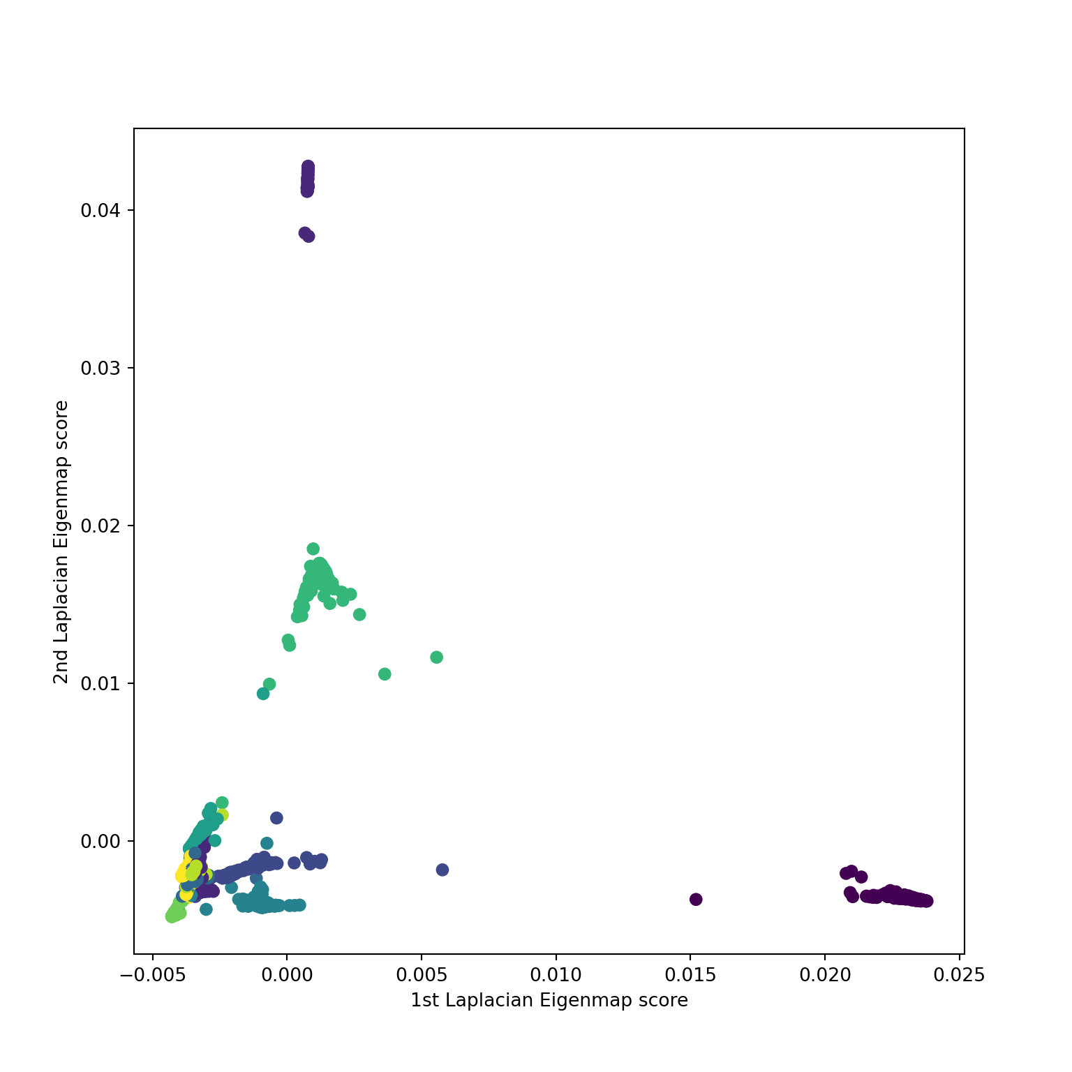
Diffusion based graph distances
- For symmetric \(W\), let
\[ A_{ij} = e^{-W_{ij}} \]
- Common choice
\[ A_{ij} = e^{-\kappa \|X[i]-X[j]\|^2_2/2}. \]
- Let’s normalize the rows
\[ T_{ij} = \frac{A_{ij}}{\sum_{k:k \sim i} A_{ik}} = \frac{A_{ij}}{\pi_{i}} = (\Pi^{-1}A)_{ij} \]
- This is a transition matrix for a Markov chain.
\[ P(X_{t+1}=j|X_{t}=i) = T_{ij}. \]
- If a chain takes a long time to get to \(j\) starting from \(i\), then \(j\) is far from \(i\).
- Associated to \(T\) is its generator
\[ I-T \]
- In unnormalized setting this corresponds to
\[ L = \Pi - A. \]
- We see \((I-T)1=0\) (and \(L1=0\)):
\[ (I - T)f = f(i) - \text{Avg}_{j: j \sim i} f(j) \]
- Eigenvalues of \(I-T\) are those of generalized eigenvalue problem
\[ Lf = \lambda \Pi f, \qquad \Pi^{-1/2}L\Pi^{-1/2}h = \lambda h. \]
- Eigenfunctions corresponding to small eigenvalues are smoother functions.
Kernels from graph
The matrix \(L\) is non-negative definite… as is its (formal) inverse the Green’s function. Alternatively, \(\Pi^{-1/2}L\Pi^{-1/2}\) is also non-negative definite as is its (formal) inverse.
Gives another distance based on a graph, different from geodesic distance…

|

|
Source: Belkin and Niyogi
```
Changing the cost function
Local MDS (c.f. Chen and Buja (2009), 14.9 of ESL)
Local MDS defines a proximity graph and seeks \[ \text{argmin}_{y_1, \dots, y_n} \sum_{(i,j): i \sim j} (D_{ij} - D(y)_{ij}\|_2)^2 - \tau \sum_{(i,j): i \not \sim j} D(y)_{ij} \]
Encourages points not considered close in the graph to be faraway in the Euclidean visualization / configuration.
Locally linear embedding
- Another method that directly optimizes over \(y \in \mathbb{R}^{n \times k}\).
- Given graph \(G\) (usually some number of nearest neighbors), solve for weights (\(W_{ij} \neq 0 \iff i \sim j\))
\[ \min_{W[i]:W[i]^T1=1} \|X[i] - \sum_{j:j \sim i} W_{ij} X[j]\|^2_2 \]
(The weights are an averaging operator, computing norm is similar to Laplacian…)
- With \(W\) fixed, find \(Y \in \mathbb{R}^{n \times k}\) that minimizes
\[ \sum_i\|Y[i] - \sum_{j:j \sim i}W_{ij}Y[j]\|^2_2 \]
subject to \(1^TY=0, Y^TY/n=I\). (Last constraint is non-trivial: otherwise \(Y\)=0 is the solution – uninteresting.)
- First constraint is trivial by step 1. – matrix \(I-W\) satisfies
\[ (I-W)1=0 \]
- Take next \(k\) eigenvectors (ordering eigenvalues from smallest to largest).
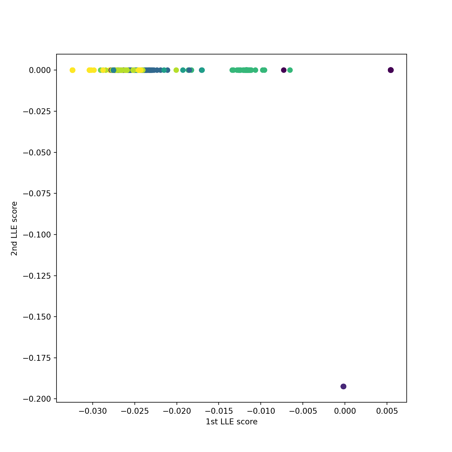
Using n_neighbors=5
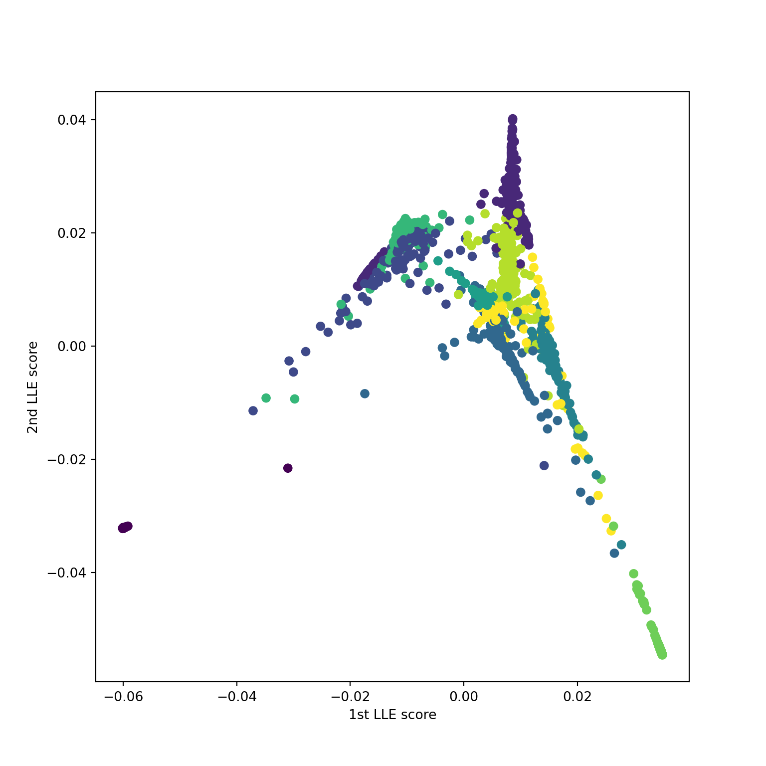
Using n_neighbors=10
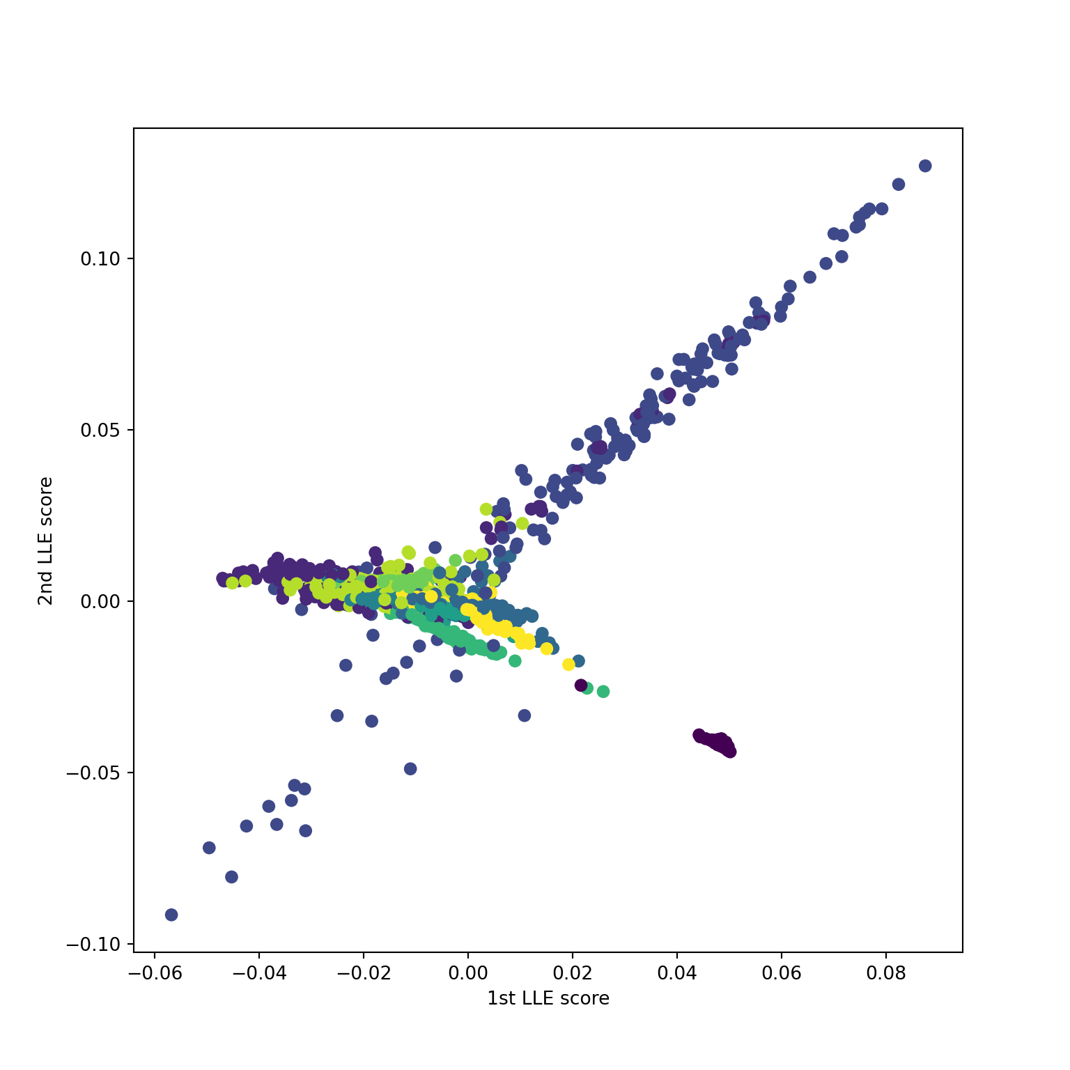
Using n_neighbors=15

Source: ESL