Multivariate regression
Multiple linear regression

Response matrix: \(Y \in \mathbb{R}^{n \times q}\)
Design matrix: \(X \in \mathbb{R}^{n \times p}\)
MKB swaps \(p\) and \(q\). Here \(p\) always refers to features.
Model
\[ Y_{n \times q} = X_{n \times p} B_{p \times q} + \epsilon_{n \times q}, \qquad \epsilon \sim N(0, I_{n \times n} \otimes \Sigma_{q \times q}) \]
- MKB uses \(U\) instead of \(\epsilon\).
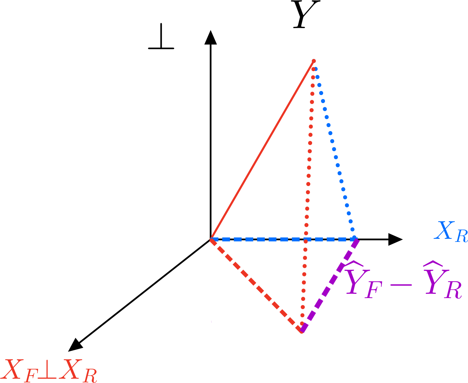
Geometry of OLS still applies
Soils example
Estimation of \(B\)
Negative log-likelihood
\[ \begin{aligned} \ell(B,\Sigma) &= - \log L(B,\Sigma|X,Y) \\ &= \frac{n}{2} \log |2\pi\Sigma| + \frac{1}{2} \text{Tr}\left(\Sigma^{-1}(Y-XB)^T(Y-XB)\right) \\ \end{aligned} \]
- As in one-sample problem
\[ \frac{1}{t}\left[ \ell(B + t\Delta,\Sigma) - \ell(B, \Sigma) \right] = \frac{1}{2}\text{Tr}\left(\Sigma^{-1} \left(\Delta^TX^T(Y-XB) + (Y-XB)^TX\Delta \right) \right) + O(t^2) \]
- Score equation (assuming \(\Sigma >0\))
\[ X^T(Y-X\hat{B}) = 0 \qquad \implies \hat{B} = (X^TX)^{-1}X^TY \in \mathbb{R}^{p \times q} \]
Estimation of \(\Sigma\)
\[ \hat{\Sigma}_{MLE} = \frac{1}{n}Y^T(I-P_F)Y, \qquad P_F = X(X^TX)^{-1}X^T \]
- For \(\hat{\Sigma}_{MLE}>0\) we need \(\text{rank}(I-P_F) \geq q\) which is generic if \(n-p \geq q\).
Unbiased estimate
\[ \hat{\Sigma} = \frac{1}{n-p} Y^T(I-P_F)Y \]
Minimized (negative) log-likelihood
- As in one-sample problem we see
\[ \ell(\hat{B}, \hat{\Sigma}_{MLE}) = \frac{n}{2} \log \det(2\pi\hat{\Sigma}) + \frac{n}{2} \]
- Criterion for use e.g. in AIC, BIC…
LRT (up to multiplicative factor)
\[ \log \det(\hat{\Sigma}_R^{-1} \hat{\Sigma}_F) \]
Distribution results
Fairly easy to check:
\(\hat{B} \sim N(B, (X^TX)^{-1} \otimes \Sigma)\)
\((n-p) \hat{\Sigma} \sim \text{Wishart}(n-p, \Sigma)\)
\(\hat{B}\) independent of \(\hat{\Sigma}\)
Sums of squares matrices
Set \(I-P_C=I-\frac{1}{n}11^T\).
Just like
lmbut matrices…
\[ \begin{aligned} \textrm{SST}_{q \times q} &= Y^T(I-P_C)Y \\ \textrm{SSE}_{q \times q} &= Y^T(I-P_F)Y \\ \textrm{SSR}_{q \times q} &= Y^T(P_F-P_C)Y \\ \textrm{SST} &= \textrm{SSE}+\textrm{SSR} \end{aligned} \]
Analogy of \(F\)-test in summary.lm
Typically first column of \(X\) is \(1\).
Usual \(F\) test is of
\[ H_0: E[Y|X] = 1\mu^T \]
- Natural matrix to consider
\[ HE^{-1} \qquad H=\textrm{SSR}, \qquad E=\textrm{SSE} \]
Likelihood ratio test statistic
\[ \log\det( \textrm{SST}^{-1}\; \textrm{SSE}) = - \log \det((H + E)^{-1}E) \]
Test statistic: Wilks’ Lambda (LRT/n), Roy’s maximum root: largest eigenvalue, etc.
Section 6.5.4. MKB use \((H+E)^{-1}E\) as analog of \(1-R^2\): a Beta matrix under \(H_0\)
Inference
General linear hypothesis
\[ H_0:C_{r \times p} B_{p \times q} A_{q \times c} = h_{r \times c} \]
Special case
- To test hypotheses of the form
\[ H_0:CB=0 \]
- Key quantities are sums of squares matrices
\[ \begin{aligned} H &= SSE(R) - SSE(F) \\ &= Y^T(P_F-P_R)Y\\ E &= SSE(F) \\ &= Y^T(I-P_F)Y\\ \end{aligned} \]
with
\[ P_F-P_R = X(X^TX)^{-1}C^T(C(X^TX)^{-1}C^T)^{-1}C(X^TX)^{-1}X^T \]
Where does \(P_F-P_R\) come from?
Type III MANOVA
Sanity check for Block
Compute the LRT
Types of Sums of Squares
Here is a good reference
For \(q=1\),
Rreturns Type I sums of squares. Arguably, Type II or III is more natural.When no interactions present, Type II will agree with Type III, otherwise can differ: see
DepthandContourbelow.When designs are balanced, Type I can agree with Type II.
Type I vs. Type 2 & 3
Other test statistics: Roy’s maximum root
- Based on the union-intersection principle using the family
\[ \begin{aligned} H_{0,a}&: CBa = 0 \\ H_0 &= \cap_{a} H_{0,a} \end{aligned} \]
- For each \(a\) we can test \(H_{0,a}\) with an \(F\)-test
\[ \frac{1}{k a^TEa / (n-p)}(C\widehat{B}a)^T \left(C(X^TX)^{-1}C^T \right)^{-1} C\widehat{B}a = \frac{n-p}{k} \frac{a^THa}{a^TEa} \]
- Ignoring factor \((n-p)/k\) we then maximize over \(a\)
\[ \begin{aligned} \sup_a \frac{a^THa}{a^TEa} &= \sup_b \frac{b^TE^{-1/2}HE^{-1/2}b}{b^Tb} \\ &= \lambda_1(HE^{-1}) \end{aligned} \]
Computing Roy’s maximum root
Hotelling-Lawley trace
- Test statistic: \(\text{Tr}(HE^{-1})\).
Pillai-Bartlett trace
- Test statistic: \(\text{Tr}((I + HE^{-1})^{-1})) = \text{Tr}(E(E+H)^{-1}).\)
Finding Sum of Squares from Manova
Tests about different responses
- We might sometimes be interested in testing a hypothesis of the form
\[ H_0: BM = 0 \]
- For example, the hypothesis that all \(q\) coefficient vectors are identical
\[ H_0: B = \gamma 1^T \quad \iff \quad B\left(I - \frac{1}{q} 11^T \right) = 0 \]
Reduced response
- In this case, we use response vector \(\widetilde{Y}=YM\) and the model
\[ \widetilde{Y} = X\widetilde{B} + \widetilde{\epsilon} \]
Our hypothesis here can be expressed as \(\widetilde{B}=0\).
Hence, the relevant sums of squares are
\[ \begin{aligned} \tilde{H} &= (YM)^TP_FYM \tilde{E} &= (YM)^T(I-P_F)YM \\ \end{aligned} \]
Combining both types of tests
- To test \(H_0: CBM=0\), we use
\[ \begin{aligned} H &= (YM)^T(P_F-P_R)YM \\ E &= (YM)^T(I-P_F)YM \\ \end{aligned} \]
Affine shifts
Finally, suppose \(h \neq 0\)
For this, take any fixed \(B_0 \in H_0\) such that \(CB_0M=h\) and set
\[ \widetilde{Y} = Y - XB_0 | X \sim N(X(B-B_0), I \otimes \Sigma) = N(X\Delta, I \otimes \Sigma) \]
with \(\Delta=B-B_0\).
- Our null is now \(H_0:C\Delta M=0\) and we can use
\[ \begin{aligned} H &= (\widetilde{Y}M)^T(P_F-P_R)\widetilde{Y}M \\ E &= (\widetilde{Y}M)^T(I-P_F)\widetilde{Y}M \\ \end{aligned} \]