Low-rank approximation
\[
\text{minimize}_{A \in \mathbb{R}^{n \times k},B \in \mathbb{R}^{q \times k}}
\|R_cX-AB^T\|^2_F
\]
with
\[
R_c = \left(I - \frac{1}{n}11^T\right)
\]
This is reduced rank regression objective with \(\tilde{Y}=R_cX\) , \(\tilde{X}=I\) , \(\Sigma=I\) .
Going forward, we’ll somtimes drop \(R_c\) by assuming that \(R_cX=X\) , i.e. that it has already been centered.
Solution
Our reduced-rank regression solution told us to look at \(\tilde{W}\) , \(k\) leading eigenvectors of
\[
XX^T
\]
\[
\begin{aligned}
\tilde{A} &= \tilde{W} \\
\tilde{B} &= X^T\tilde{A}(\tilde{A}^T\tilde{A})^{-1} \\
&= X^T\tilde{A}
\end{aligned}
\]
Relation to SVD
Given matrix \(M \in \mathbb{R}^{n \times p}\) (assume \(n>p\) ) there exists an SVD
\[
M = U_{n \times p} D_{p \times p} V_{p \times p}^T
\]
Properties
\[
\begin{aligned}
U^TU &= I_{p \times p} \\
D &= \text{diag}(d_1 \geq d_2 \geq \dots \geq d_p \geq 0) \\
V^TV &= \text{I}_{p \times p}
\end{aligned}
\]
\[
MM^T = UD^2U^T
\]
\[
M^TM = VD^2V^T.
\]
\[
M^TU = VD
\]
Can absorb \(D\) into \(U\) by writing
\[
M = (UD)V^T
\]
Back to reduced rank
Our reduced rank solution with \(X=UDV^T\) picks
\[
\begin{aligned}
\hat{A} &= U[,1:k] \\
\hat{B} &= D[1:k,1:k] V[,1:k]^T
\end{aligned}
\]
More common to think of rank-\(k\) PCA in terms of first \(k\) scores
\[
U[,1:k] D[1:k,1:k]
\]
and loadings
\[
V[,1:k]
\]
A second motivation
Could also consider the problem
\[
\text{minimize}_{A \in \mathbb{R}^{p \times k}, B \in \mathbb{R}^{p \times k}} \|X - XAB^T\|^2_F
\]
Maximal variance
Minimizing first over \(A\) , we see this is equivalent to solving this problem
\[
\text{minimize}_{P_k} \|X - XP_k\|^2_F
\]
where \(P_k\) is a projection matrix of rank \(k\) .
Equivalently, we solve (recall \(R_cX=X\) )
\[
\text{minimize}_{P_k} \text{Tr}(X^TR_cX) - \text{Tr}(P_kX^TR_cXP_k)
\]
\[
\text{maximize}_{P_k} \text{Tr}(P_kX^TR_cXP_k)
\]
Rank \(k\) PCA captures \(k\) dimensional subspace of features that maximizes variance…
Population version
The maximizing variance picture lends itself to a population version
Thinking of rows of \(X\) as IID with law \(F\) , let \(\Sigma = \text{Var}_F(X[1,])\)
\[
\text{minimize}_{P_k} \text{Tr}(\Sigma) - \text{Tr}(P_k\Sigma P_k) \iff \text{maximize}_{P_k} \text{Tr}(P_k \Sigma P_k)
\]
Solution is to choose top \(k\) eigen-subspace of \(\Sigma\) …
PCA = SVD
Given data matrix \(X \in \mathbb{R}^{n \times p}\) with rows \(X[i,] \overset{IID}{\sim} F\) , the sample PCA can be described by the SVD of \(R_cX\)
As \(V\) can be thought as an estimate of \(\Gamma\) in an SVD of
\[
\text{Var}_F(X) \approx \Gamma \Lambda \Gamma^T
\]
we might write \(V = \widehat{\Gamma}\) .
Columns of \(\widehat{\Gamma}\) are the loadings of the principal components while columns of \(UD = \hat{Z}\) are the (sample) principal components scores.
Scaling
Common to scale columns of \(X\) to have standard deviation 1.
In this case, we are really computing the PCA of
\[
R_c X \text{diag}(S)^{-1}
\]
\[
S^2_{i,i} = \frac{1}{n-1}X[,i]^TR_cX[,i] = {\tt sd(X[,i])}^2
\]
Synthetic example
= 50 = 10 = matrix (rnorm (n* p), n, p)= diag (rep (1 , n)) - matrix (1 , n, n) / n= svd (R_c %*% X)= SVD_X$ u %*% diag (SVD_X$ d)= SVD_X$ v= prcomp (X, center= TRUE , scale.= FALSE )names (pca_X)
[1] "sdev" "rotation" "center" "scale" "x"
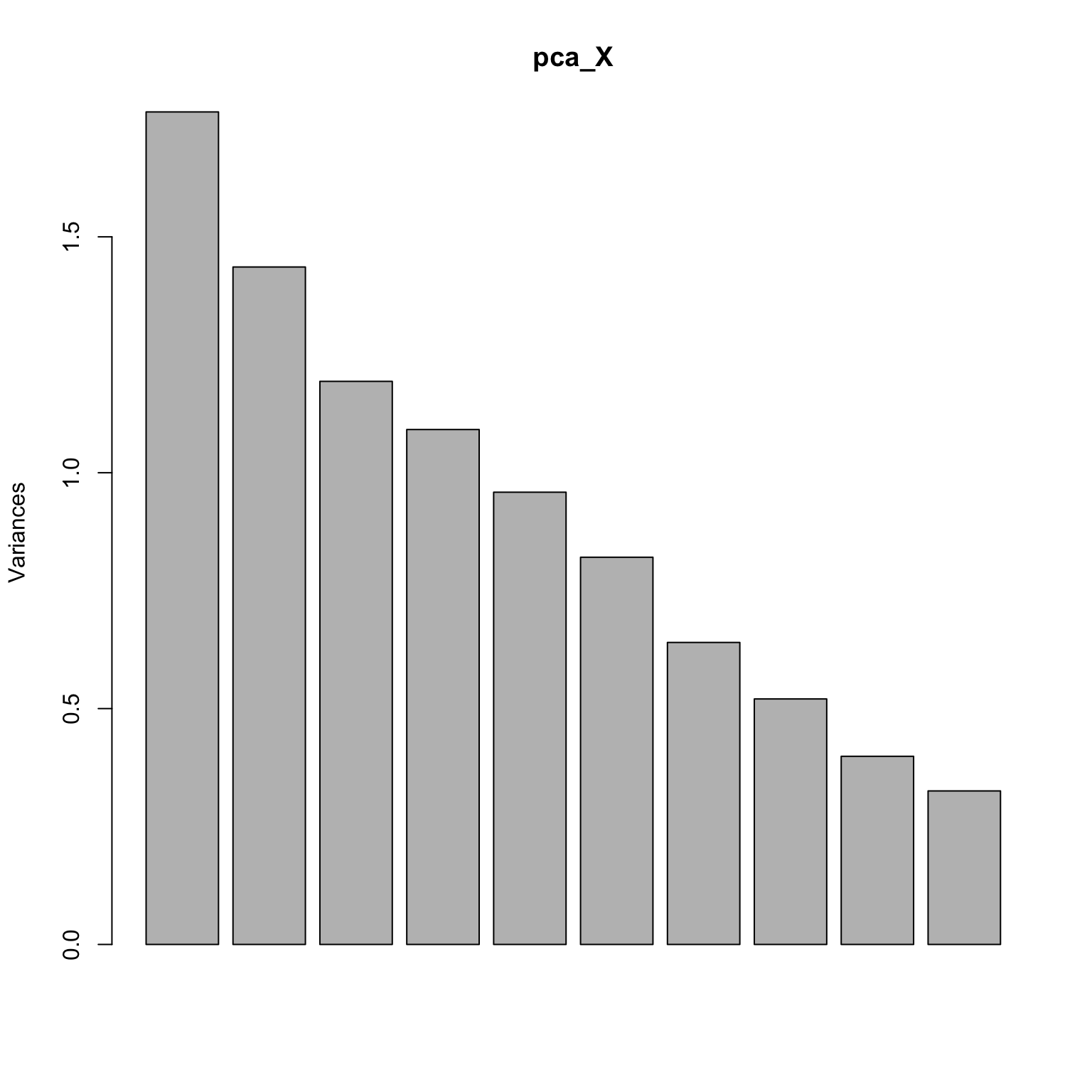
Screeplot: is there an elbow?
Check loadings
Call:
lm(formula = Gamma_hat[, 1] ~ pca_X$rotation[, 1])

Residuals:
       Min         1Q     Median         3Q        Max
-9.336e-16 -7.160e-16 -5.859e-17  4.491e-16  1.941e-15

Coefficients:
                      Estimate Std. Error    t value Pr(>|t|)
(Intercept)         -6.733e-16  3.150e-16 -2.137e+00    0.065 .
pca_X$rotation[, 1]  1.000e+00  9.962e-16  1.004e+15   <2e-16 ***
---
Signif. codes:  0 '***' 0.001 '**' 0.01 '*' 0.05 '.' 0.1 ' ' 1

Residual standard error: 9.387e-16 on 8 degrees of freedom
Multiple R-squared:      1, Adjusted R-squared:      1
F-statistic: 1.008e+30 on 1 and 8 DF,  p-value: < 2.2e-16
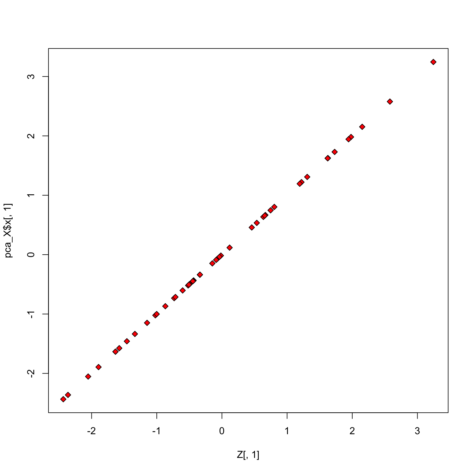
Check scores
With scaling
= 1 / (sqrt (diag (t (X) %*% R_c %*% X) / 49 ))= svd (R_c %*% X %*% diag (S_inv))= SVD_Xs$ u %*% diag (SVD_Xs$ d)= SVD_Xs$ v= prcomp (X, center= TRUE , scale.= TRUE )
Check loadings
summary (lm (Gamma_hat_s[,1 ] ~ pca_Xs$ rotation[,1 ]))
Call:
lm(formula = Gamma_hat_s[, 1] ~ pca_Xs$rotation[, 1])

Residuals:
       Min         1Q     Median         3Q        Max
-4.314e-15 -2.378e-15 -2.862e-16  1.956e-15  7.417e-15

Coefficients:
                       Estimate Std. Error    t value Pr(>|t|)
(Intercept)          -1.391e-15  1.239e-15 -1.123e+00    0.294
pca_Xs$rotation[, 1]  1.000e+00  3.917e-15  2.553e+14   <2e-16 ***
---
Signif. codes:  0 '***' 0.001 '**' 0.01 '*' 0.05 '.' 0.1 ' ' 1

Residual standard error: 3.698e-15 on 8 degrees of freedom
Multiple R-squared:      1, Adjusted R-squared:      1
F-statistic: 6.516e+28 on 1 and 8 DF,  p-value: < 2.2e-16
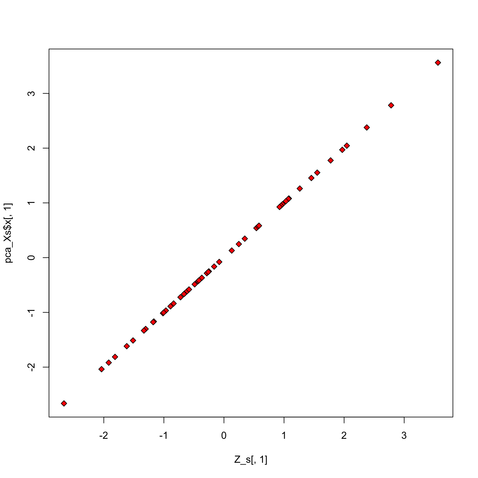
Check scores
Some example applications
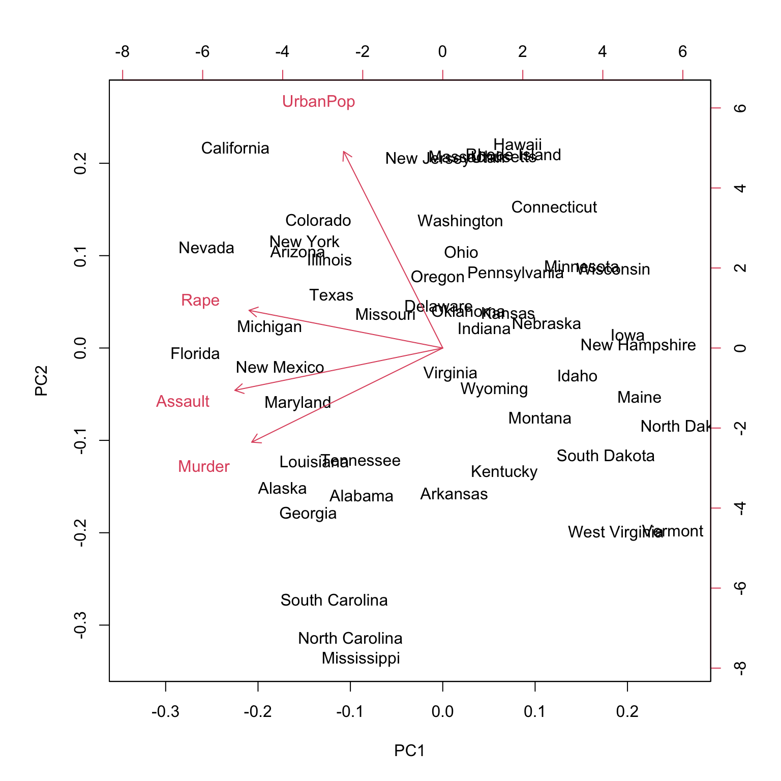
USArrests data
= prcomp (USArrests, scale = TRUE )names (pr.out)
[1] "sdev" "rotation" "center" "scale" "x"
Output of prcomp
The center and scale components correspond to the means and standard deviations of the variables that were used for scaling prior to computing SVD
  Murder  Assault UrbanPop     Rape
   7.788  170.760   65.540   21.232
   Murder   Assault  UrbanPop      Rape
 4.355510 83.337661 14.474763  9.366385
Rotation / loading
                PC1        PC2        PC3         PC4
Murder   -0.5358995 -0.4181809  0.3412327  0.64922780
Assault  -0.5831836 -0.1879856  0.2681484 -0.74340748
UrbanPop -0.2781909  0.8728062  0.3780158  0.13387773
Rape     -0.5434321  0.1673186 -0.8177779  0.08902432
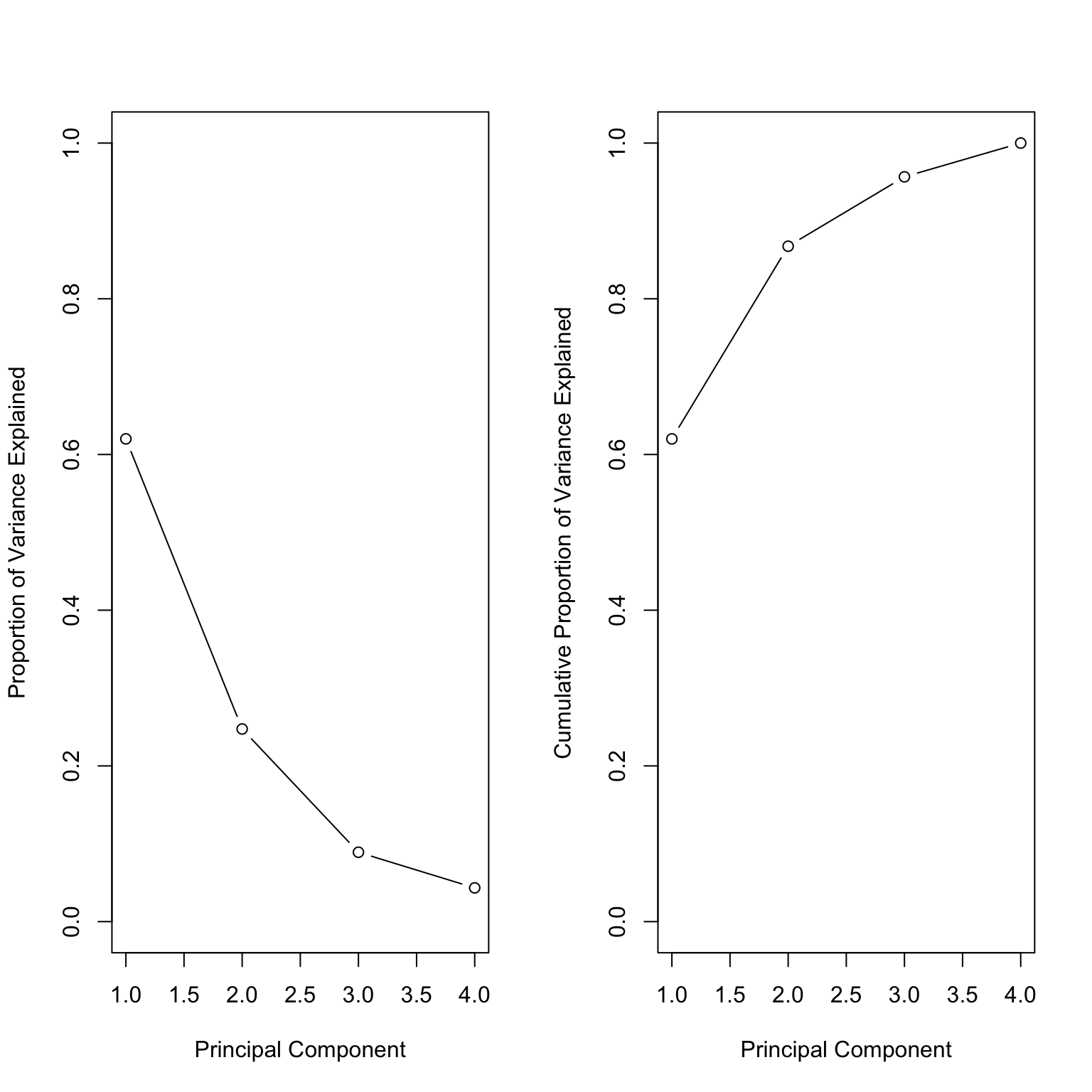
Biplot
Variance explained
[1] 1.5748783 0.9948694 0.5971291 0.4164494
= pr.out$ sdev^ 2
[1] 2.4802416 0.9897652 0.3565632 0.1734301
= read.csv ('https://archive.ics.uci.edu/ml/machine-learning-databases/voting-records/house-votes-84.data' , header= FALSE )head (voting_data)
          V1 V2 V3 V4 V5 V6 V7 V8 V9 V10 V11 V12 V13 V14 V15 V16 V17
1 republican  n  y  n  y  y  y  n  n   n   y   ?   y   y   y   n   y
2 republican  n  y  n  y  y  y  n  n   n   n   n   y   y   y   n   ?
3   democrat  ?  y  y  ?  y  y  n  n   n   n   y   n   y   y   n   n
4   democrat  n  y  y  n  ?  y  n  n   n   n   y   n   y   n   n   y
5   democrat  y  y  y  n  y  y  n  n   n   n   y   ?   y   y   y   y
6   democrat  n  y  y  n  y  y  n  n   n   n   n   n   y   y   y   y
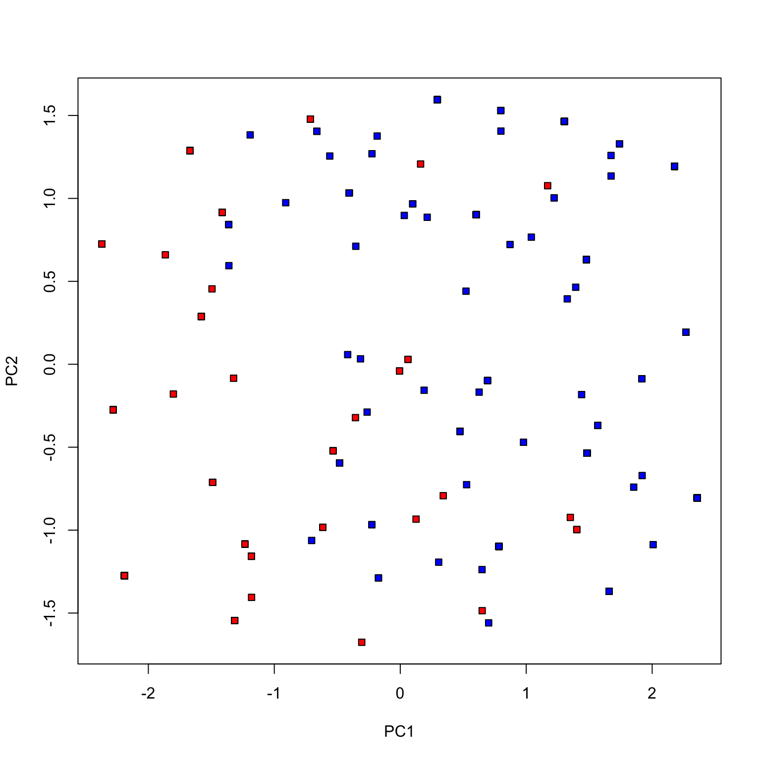
= c ()for (i in 2 : 7 ) {= factor (voting_data[,i], c ('n' , '?' , 'y' ), ordered= TRUE )= cbind (voting_X, as.numeric (voting_data[,i]))= prcomp (voting_X, scale.= TRUE )= voting_data[,1 ] == 'democrat' = ! dem
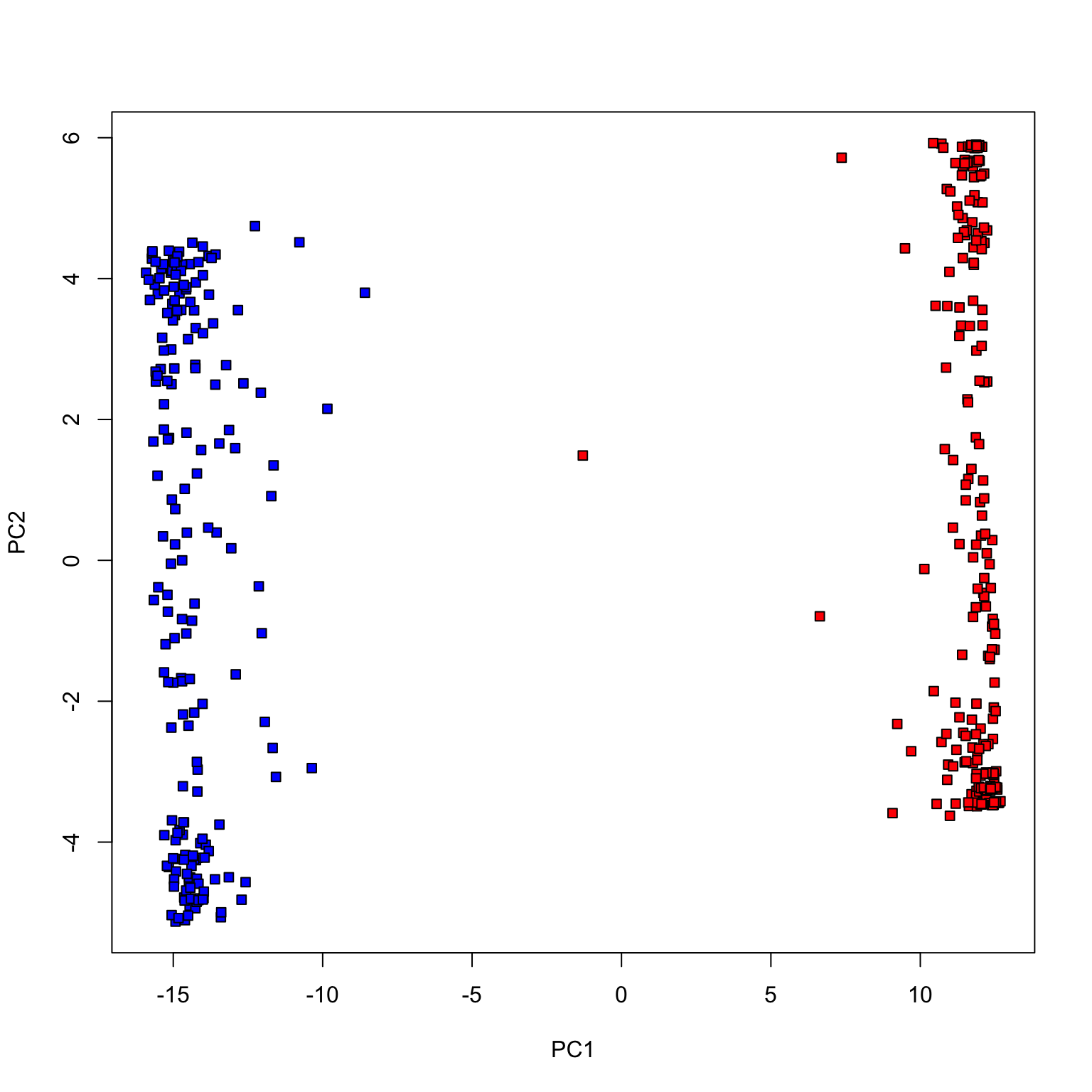
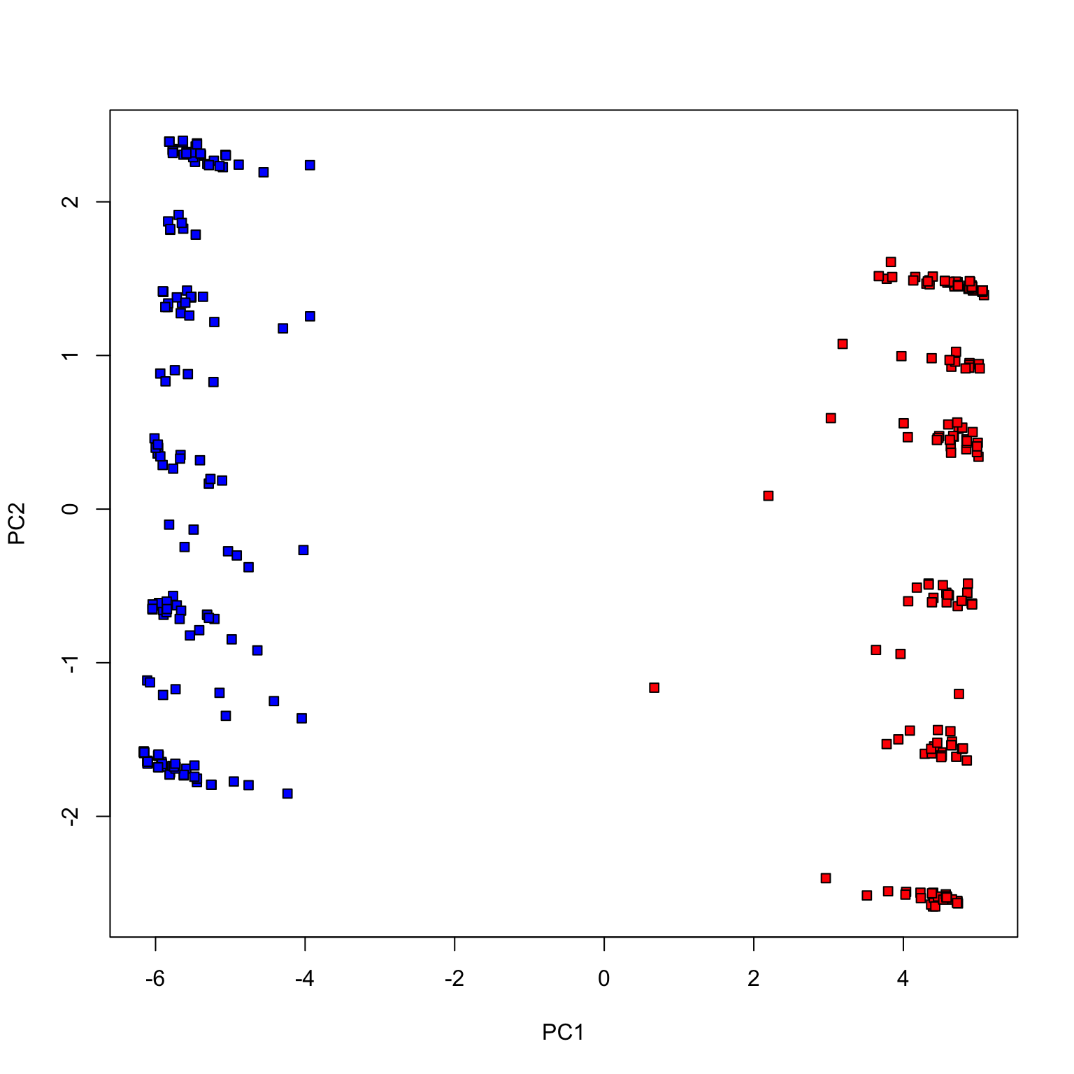
plot (pca_votes$ x[,1 ], pca_votes$ x[,2 ], type= 'n' , xlab= 'PC1' , ylab= 'PC2' )points (pca_votes$ x[dem, 1 ], pca_votes$ x[dem, 2 ], pch= 22 , bg= 'blue' )points (pca_votes$ x[repub, 1 ], pca_votes$ x[repub, 2 ], pch= 22 , bg= 'red' )
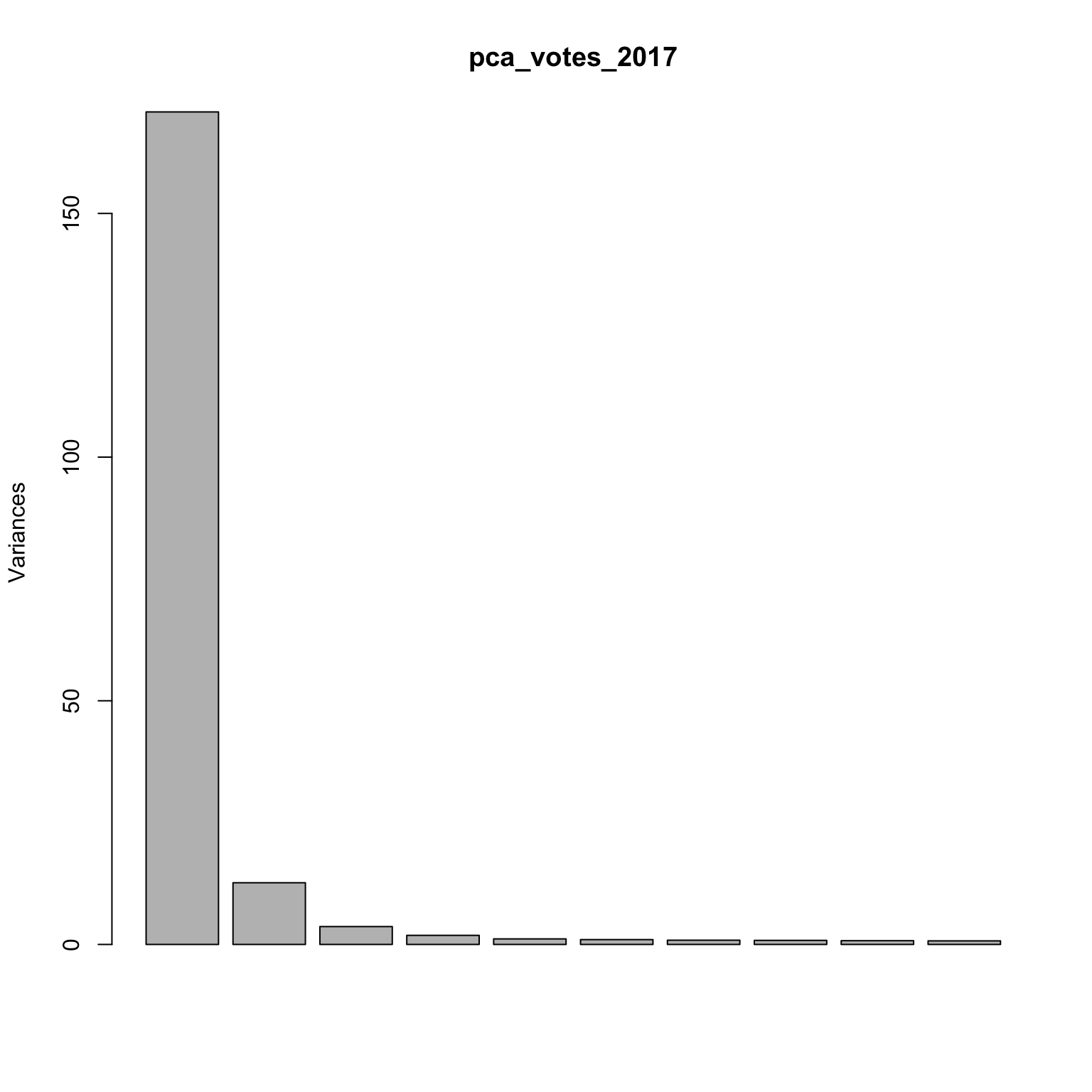
Congress of 2017
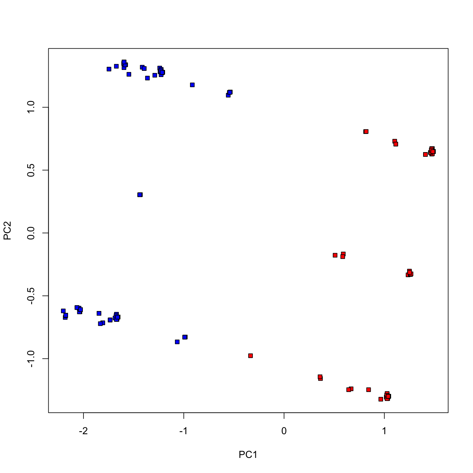
Fewer votes (randomly chosen 100 votes)
Fewer votes (randomly chosen 20 votes)
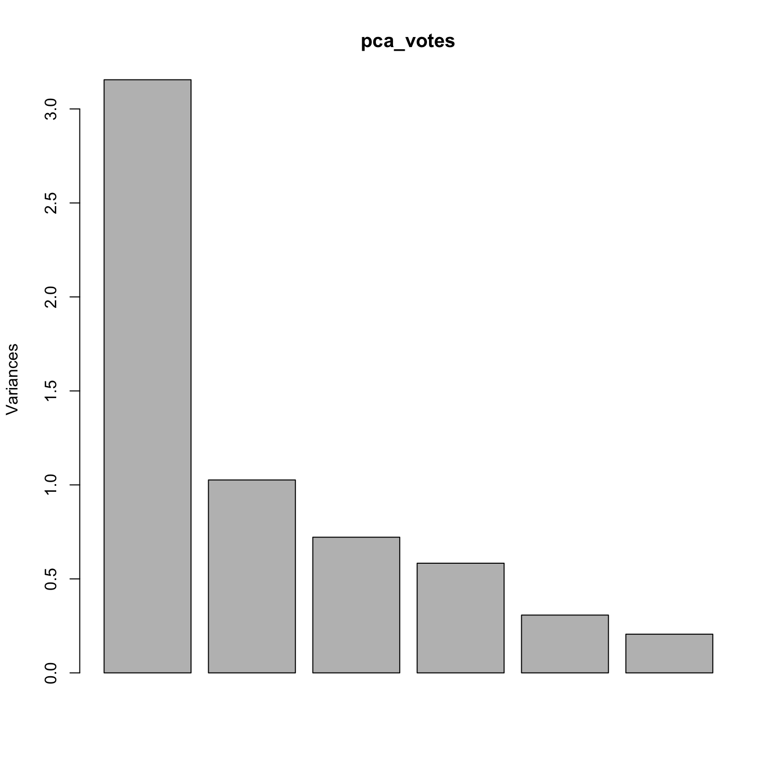
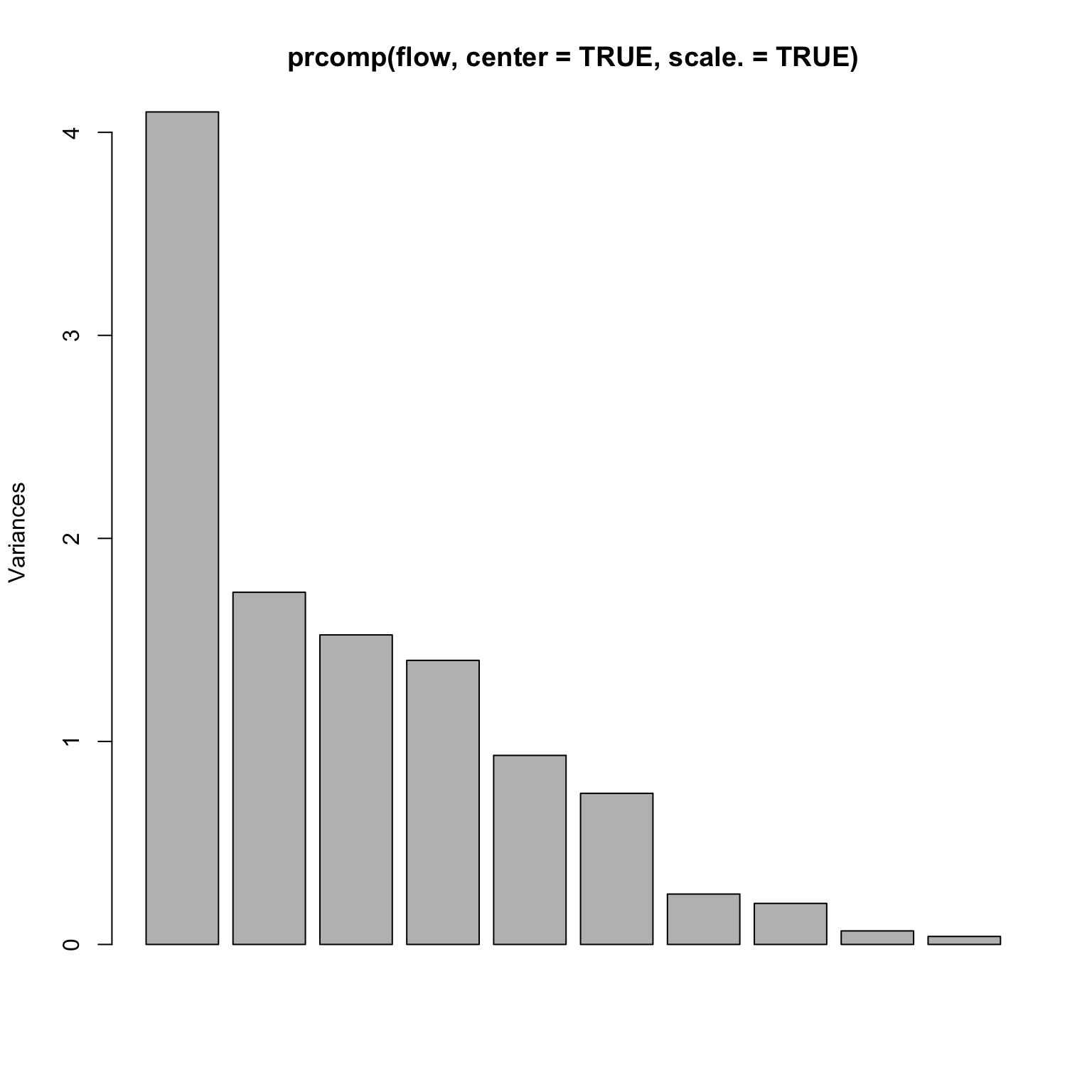
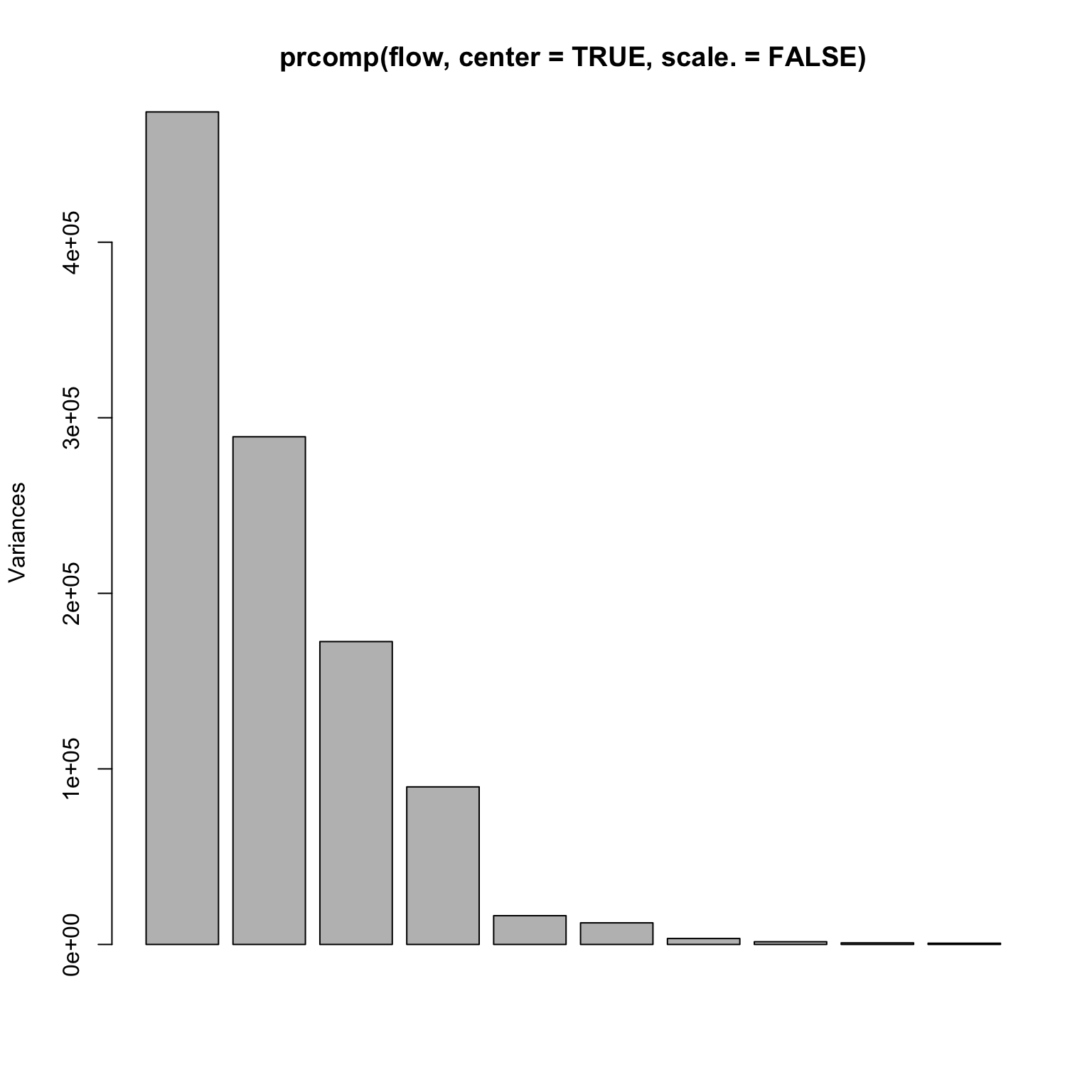
= read.table ('http://www.stanford.edu/class/stats305c/data/sachs.data' , sep= ' ' , header= FALSE )dim (flow)plot (prcomp (flow, center= TRUE , scale.= TRUE ))
A rank 4 model?
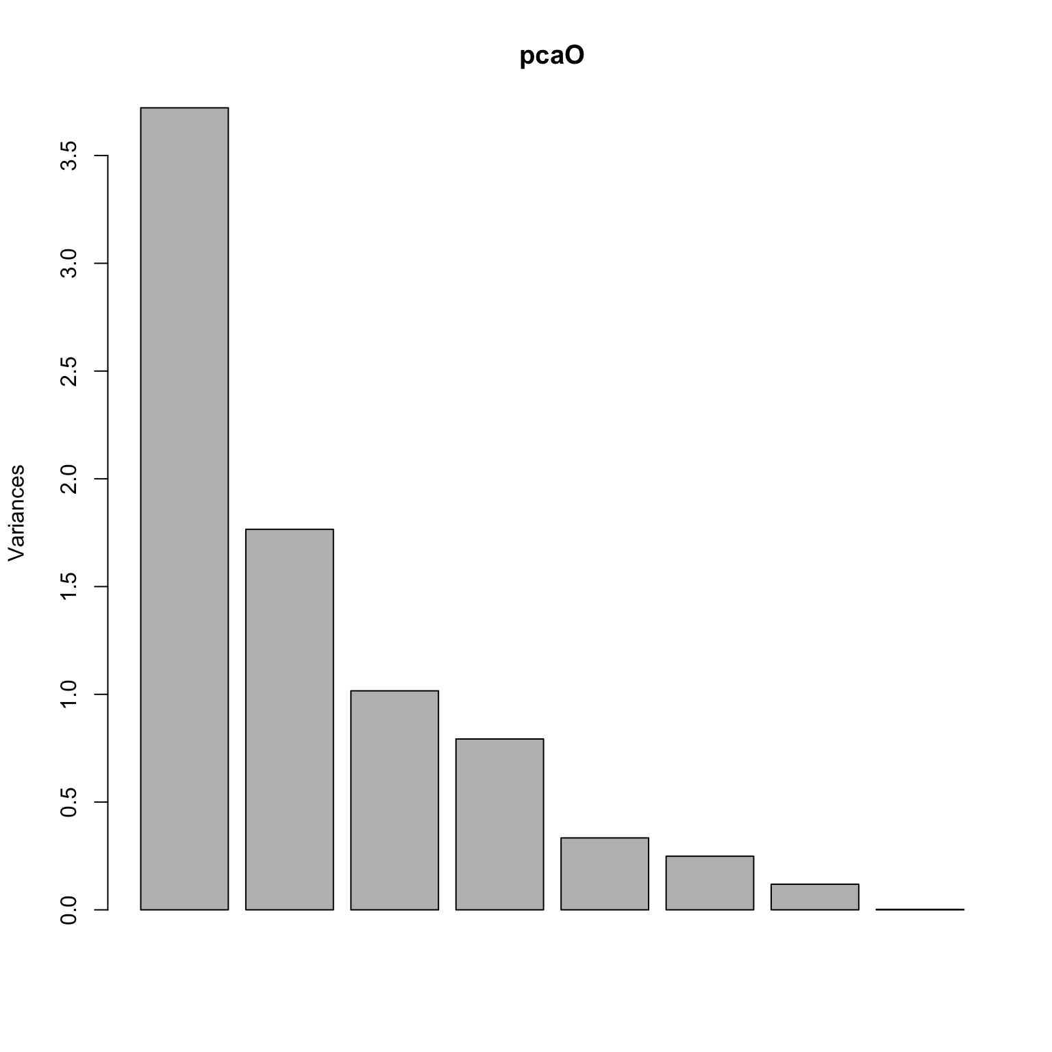
Olive oil data
library (pdfCluster)data (oliveoil)= oliveoil[,3 : 10 ]= prcomp (featO, scale.= TRUE , center= TRUE )plot (pcaO)
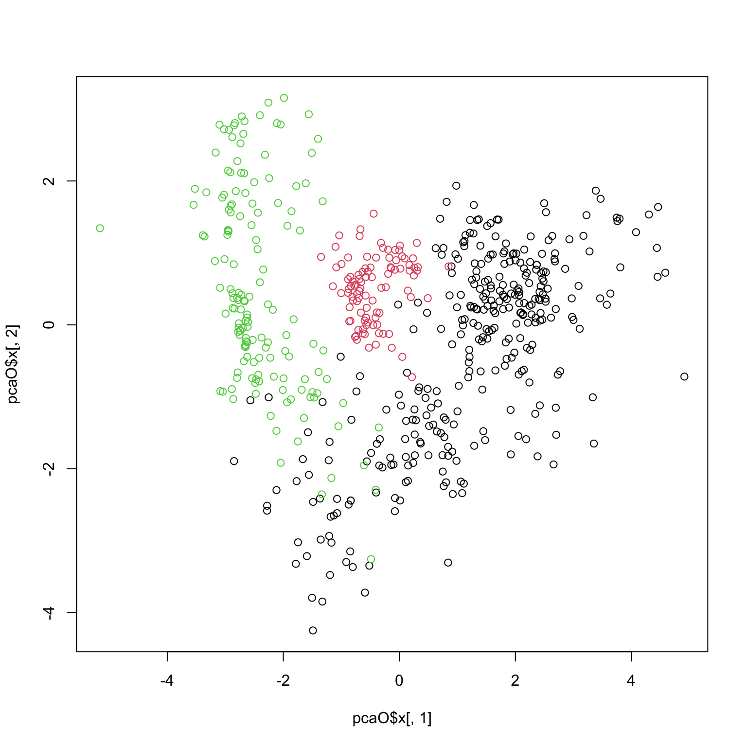
plot (pcaO$ x[,1 ], pcaO$ x[,2 ], col= oliveoil[,'macro.area' ])
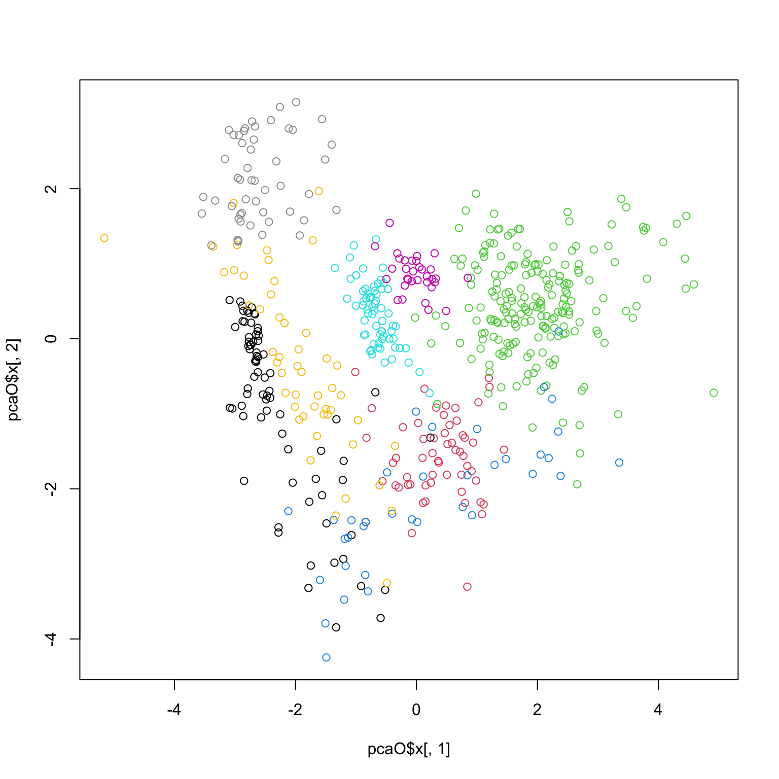
plot (pcaO$ x[,1 ], pcaO$ x[,2 ], col= oliveoil[,'region' ])