Penalized Discriminant Analysis
Penalized Discriminant Analysis
Builds on the connection between CCA and LDA
We will follow (in some fashion):
- Flexible Discriminant Analysis Hastie, Tibshirani, Buja (1993)
- Penalized Discriminant Analysis Hastie, Buja, Tibshirani (1995)
- Chapter 12 of ESL
References refer to optimal scoring (OS), we will not…
Takeaways
- Turns regression procedure
Y ~ Xinto a discriminant classifierY: one-hot encoding of classesX: features
- Ideal for ridge-type smoothing
Outline
All of multivariate analysis:
lm(Y ~ X)andsvd()Laplacians and smoothing
Most of the time \(Y\), \(X\) will be random vectors rather than data matrices (exceptions will hopefully be clear from context)
Smooth LDA for digits
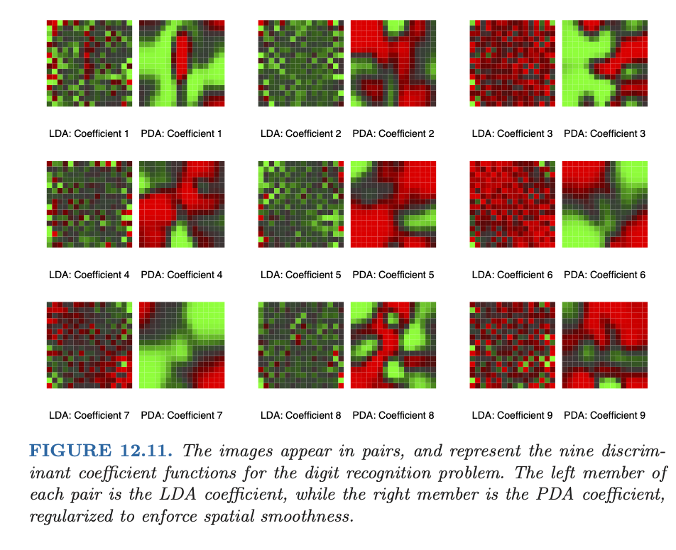
(Source: ESL)
CCA’s generalized eigenvalue problems
- In CCA, we looked at eigen-decompositions of
\[ \Sigma_{YY}^{-1/2} \Sigma_{YX} \Sigma_{XX}^{-1} \Sigma_{XY} \Sigma_{YY}^{-1/2} = U_Y \Lambda^2 U_Y' \]
- Setting \(A_Y'=\Sigma_{YY}^{-1/2}U_Y\) yields solutions
\[ \Sigma_{YX} \Sigma_{XX}^{-1} \Sigma_{XY} a_{Y,i} = \lambda^2_i a_{Y,i}, 1 \leq i \leq m=\text{rank}(\Sigma_{XY}) \]
with
\[ a_{Y,i}'\Sigma_{YY}a_{Y,j} = \delta_{ij}. \]
- Yielded the canonical variates
\[ Z_{Y,i} = a_{Y,i}'Y, \qquad Z_{Y,i}'Z_{Y,j} = \delta_{ij} \]
Matrix form
- For non-singular \(A_X, A_Y\)
\[ \begin{aligned} Z_Y &= A_Y Y \\ Z_X &= A_X X \end{aligned} \]
Projection version
- Let \(P_X, P_Y\) denote the correspond projections (either sample or population) of centered \(X, Y\)
Population version
- \(P_X\) projection onto \(\text{span}((X_i - \mathbb{E}[X_i]), 1 \leq i \leq p)\) in \(L^2(\mathbb{P})\)
Sample version
- With \(R_C=I-P_C=I-n^{-1}11'\), we see that
\[\hat{P}_X = RX(X'RX)^{-1}X'R\]
projects onto \(\text{span}((X_i - \mathbb{E}[X_i]), 1 \leq i \leq p)\) in \(L^2(\widehat{\mathbb{P}})\)
Canonical variates
\[ P_XP_Y = \sum_{i=1}^{m} \lambda_i Z_{X,i} Z_{Y,i}' = \sum_{i=1}^m \lambda_i Z_{X,i} \otimes Z_{Y,i}, \qquad m = \text{rank}(\Sigma_{XY}) \]
Regression in terms of canonical variates
- Straightforward to check
\[ \begin{aligned} \Lambda &= \text{argmin}_{L} \mathbb{E}[\|Z_Y - L'Z_X\|^2_2] \\ \end{aligned} \]
\(\implies\) \(X\) uses \(\Lambda Z_X\) to predict \(Z_Y\)
Given nominal OLS fits \(\hat{Y}=B'X\) (\(B=\Sigma_{XX}^{-1}\Sigma_{XY}\)) we can conclude that \(A_YB'X=A_Y\hat{Y}\) predicts \(Z_Y\).
\(\implies\) \(A_YB'X=\Lambda Z_X\)!
Reduced rank regression
- Claim:
\[ \text{argmin}_{L: \text{rank}(L)=k} \mathbb{E}[\|Z_Y - L'Z_X\|^2_2] = \text{diag}(\lambda_1, \dots, \lambda_k, 0, \dots, 0) \overset{def}{=} \Lambda_k \]
- Almost OS of Hastie et al.
Regression in original space
- By equivariance of regression
\[ \text{argmin}_B \mathbb{E}[(Y-BX)\Sigma_{YY}^{-1}(Y-BX)] = A_Y^{-1}\Lambda A_X \]
Reduced rank
\[ \text{argmin}_{B:\text{rank}(B)=k} \mathbb{E}[(Y-BX)\Sigma_{YY}^{-1}(Y-BX)] = A_Y^{-1}\Lambda_k A_X \]
Connection to multivariate linear regression
- Consider regression
Y ~ X(burying1within \(X\))
\[ \mathbb{R}^q \ni Y|X \sim N(B'X, \Sigma) \]
- Recall the sample quantities
\[ \begin{aligned} \textrm{SST}_{q \times q} &= Y^T(I-P_C)Y \\ \textrm{SSE}_{q \times q} &= Y^T(I-P_F)Y \\ \textrm{SSR}_{q \times q} &= Y^T(P_F-P_C)Y \\ &= \hat{Y}'(P_F-P_C)\hat{Y}\\ &= \hat{Y}'(I-P_C)Y\\ \textrm{SST} &= \textrm{SSE}+\textrm{SSR} \end{aligned} \]
- Population quantities
\[ \begin{aligned} Q^Y_T &= \mathbb{E}[(Y- \mathbb{E}[Y])(Y- \mathbb{E}[Y])'] \\ Q^Y_E &= \mathbb{E}[(Y- BX)(Y- BX)'] \\ Q^Y_R &= \mathbb{E}[(\mathbb{E}[Y]- BX)(\mathbb{E}[Y]- BX)'] \\ &= \mathbb{E}[(\mathbb{E}[Y]- BX)Y'] \\ \end{aligned} \]
CCA eigenvalues and multivariate regression
- The generalized eigenvalue problem we considered above is
\[ Q^Y_R v = \lambda^2 Q^Y_T v \]
\(\implies\) \(\Lambda^2\) are eigenvalues of \(H(H+E)^{-1}\)
Swapping \(X\) and \(Y\) shows these are the same eigenvalues for the regression
X ~ Y(with \(Q^X_T, Q^X_E, Q^X_R\))In LDA model
X ~ Yreally is multivariate linear regression…
So what? (Back to LDA)
Two key observations (implicit / semi-explicit in ESL)
\(\Sigma_{YY}^{-1/2}Q_R\Sigma_{YY}^{-1/2}= U_Y\Lambda^2 U_Y'\)
\(\implies\) we can find \(A_Y=\Sigma_{YY}^{-1/2}U_Y\)
Given \(A_Y\) and \(BX\) we can assume \(A_YB'X\) predicts \(A_YY=Z_Y\).
Combiined: \(\implies\) \(A_YB'X = \Lambda Z_X, \iff Z_X=\Lambda^{-1}A_YB'X = \Lambda^{-1}A_Y\hat{Y}(X)\)
Fisher’s discriminants from canonical variates
- CCA (equivalent) eigenproblems (with \(a_{i,X}'\Sigma_{XX} a_{j,X} = \delta_{ij}\))
\[ \begin{aligned} \Sigma_{XX} a_{i,X} &= \lambda_i^2 \Sigma_{XY}\Sigma_{YY}^{-1} \Sigma_{YX} a_{i,X} \\ \Sigma_{X,T} a_{i,X} &= \lambda_i^2 \Sigma_{X,B} a_{i,X} \\ Q^X_T a_{i,X} &= \lambda_i^2 Q^X_R a_{i,X} \\ \end{aligned} \]
- LDA (equivalent) eigenproblems
\[ \begin{aligned} \Sigma_{X,W} \alpha_{i,X} &= \bar{\lambda}_i^2 \Sigma_{X,B} \alpha_{i,X} \\ Q^X_E \alpha_{i,X} &= \bar{\lambda}_i^2 Q^X_R \alpha_{i,X} \end{aligned} \]
- Desiderata: find eigenvectors \(\alpha_i\) and normalize \(\alpha_{i,X}'\Sigma_{X,W}\alpha_{j,X} = \delta_{ij}\)
Equivalence of eigenproblems
Claim
- We can take
\[ \begin{aligned} \bar{\lambda}_i^2 &= 1 - \lambda_i^2 \\ \alpha_{i,X} &= \frac{1}{\sqrt{1 - \lambda_i^2}}a_{i,X} \\ \end{aligned} \]
Proof of claim
Eigenvalue
\[ (Q_E + Q_R) a_i = \lambda^2 Q_R a_i \iff Q_E a_i = (1 - \lambda^2) Q_R a_i \]
Aside
- \(\implies\) reduced rank regression with \(Q_T\) is equivalent to using \(Q_E\): (c.f. exercise 3.22 of ESL)
Normalization
\[ \begin{aligned} \alpha_i'Q_E\alpha_i &= \frac{1}{1 - \lambda_i^2} \cdot a_i'Q_Ea_i \\ &= \frac{1}{1 - \lambda_i^2} \left(a_i'(Q_R+Q_E)a_i - a_i'Q_Ra_i\right) \\ &= \frac{1}{1 - \lambda_i^2} \left(a_i'Q_Ta_i - a_i'Q_Ra_i\right) \\ &= \frac{1}{1 - \lambda_i^2} \left(a_i'Q_Ra_i - \lambda_i^2 a_i'Q_Ta_i\right) \\ &= 1 \end{aligned} \]
Sample version (almost)
For one-hot data
Y, fitlm(Y ~ X)and formY_hat = predict(X)Compute
\[ \text{SSR} = Y'\hat{Y} - n \hat{\pi} \hat{pi}' \]
- Compute eigendecomposition
\[ (\text{SST}/n)^{-1/2}( \text{SSR}/n)(\text{SST}/n)^{-1/2} = \hat{U}_Y \hat{\Lambda}^2 \hat{U}_Y' \]
Set \(\hat{A}_Y = (\text{SST}/n)^{-1/2} \hat{U}_Y\) and adjusted fits \(\hat{Y}\hat{A}_Y'\).
Matrix of discriminant scores are
\[ \hat{V} = \hat{Y}\hat{A}_Y'(\hat{\Lambda}^2 (I-\hat{\Lambda}^2))^{-1/2} \]
- Reduced rank LDA: just use first \(k\) of the \(\hat{V}\)’s
Why almost?
For
Y, the matrix \(\text{SST}\) is rank-deficient as \(1'Y=1\) for one-hot data\(\implies \hat{\pi} \in \text{null(SST)}...\)
Solution
- Take \(\Theta_{K-1 \times K}\) whose column space is \(\text{row(SST)}\) with normalization
\[ \Theta'(D_{\hat{\pi}} - \hat{\pi}\hat{\pi}')\Theta = \Theta'D_{\hat{\pi}}\Theta = I_{K-1} \]
- Run the above procedure on
Y @ Theta.T
This is genius!
Algorithm
def fit(self, X, Y):
    self.reg_estimator.fit(X, Y)
    self.A_Y, self.L = solve_eigenproblem(Y, self.reg_estimator.predict(X))
    Z = self.transform(X)
    self.centroids = class_average(Z, Y)
    return self

def transform(self, x_new)
    yhat_new = self.reg_estimator.predict(x_new)
    return (yhat_new @ self.A_Y.T / np.sqrt(L**2 * (1 - L**2))[None,:])[:,:self.rank]

def predict(self, x_new):
    V_new = self.transform(x_new)
    return np.argmin(distance(V_new, centroids), axis=1)
A pause
Relied on (generalized) eigen decomposition of \(Y'\hat{Y}\)
This will be fine for (symmetric) linear estimators like ridge
\[ \hat{Y} = X(X'X + \gamma \cdot I)^{-1}X'Y = S_{\gamma}(Y) \]
- Easy to generalize this with a basis expansion
\[ \hat{Y} = h(X)(h(X)'h(X) + \gamma \cdot Q)^{-1} h(X)'Y \]
What does it all mean?
We motivated / derived the algorithm for
lm(Y ~ X)…For ridge, simply replace \(\Sigma_{XX}=\Sigma_{XX} + \gamma \cdot I\) above
Corresponds to regularized CCA
\[ \text{maximize}_{a_Y, a_X: a_Y'\Sigma_{YY}a_Y \leq 1, a_X'(\Sigma_{XX} + \gamma \cdot I) a_X \leq 1} a_Y'\Sigma_{YX}a_X \]
- \(\implies\) resulting \(Z_X\)’s are regularized canonical variates as are discriminants \(V\).
Back to the digits
Laplacian smoothing
The application used in ESL and Hastie, Buja, Tibshirani (1995) considers features that are \(16 \times 16\) grayscale images.
Given an undirected graph \(G=(V,E)\) (like the \(16 \times 16\) lattice in 2D), define the difference operator (after orienting edges) \(D:\mathbb{R}^V \to \mathbb{R}^E\)
\[ Df_e = Df_{[v_1,v_2]} = f_{v_2} - f_{v_1} \]
- The Laplacian (non-negative definite version) is the map \(\Delta: \mathbb{R}^V \times \mathbb{R}^V\)
\[ (\Delta f)_i = (D^*D f)_i = \sum_{e:v_1=j,v_2=i} f_i - f_j \]
- Regression problem: for digit \(d\), \(X\) the stack of images
\[ \hat{\beta}_d = (X'X + \lambda \Delta)^{-1} X'Y_d \]
Degrees of freedom
- For a (usually symmetric) linear smoother \(S:\mathbb{R}^n \to \mathbb{R}^n\)
\[ df(S) = \text{Tr}(S). \]
- Chosen to be about 40 for each digit \(d\).
Laplacian and manifold learning
Early 2000s saw an explosion in interest in Laplacians
Given noisy \(W = \mu + \epsilon \in \mathbb{R}^V\) can smooth
\[ \hat{\mu} = (I + \lambda \Delta)^{-1} W = \text{argmin}_{\mu} \|\mu - W\|^2_{\mathbb{R}^V} + \lambda \cdot \mu'\Delta \mu \]
- Prior variance is \(\Delta^{\dagger}\) (not invertible as \(\Delta 1=0\)): \(\implies\) more weight on functions with small eigenvalues
Intuition from Laplacian on \(\mathbb{R}^k\)
- For \(f \in \mathbb{C}^2(\mathbb{R}^k)\)
\[ (\Delta f)(x) = - \sum_{j=1}^k \frac{\partial^2f}{\partial^2 x_i}(x) \]
Eigenfunctions
\[ \Delta (\sin(\lambda'x)) = \|\lambda\|^2 \sin(\lambda'x) \]
- Functions with small eigenvalues are smoother than higher eigenvalues…
Generalizations
- Take \(\alpha: [0,\infty) \to [0, \infty)\) and consider
\[ \hat{\mu}_{\alpha} = \text{argmin}_{\mu} \|\mu - W\|^2_{\mathbb{R}^V} + \lambda \cdot \mu'\alpha(\Delta) \mu \]
Easy to apply given eigen decomposition of \(\Delta\)
Graph Neural Net: for graph-based features, parameterize / learn \(\alpha\)
Generators
Taking \(\alpha(v)=v\), \(\Delta\) is (discrete-time) generator of random walk on the graph…
Taking \(\alpha(v)=e^{-tv}\), \(e^{-t\Delta}\) is the transition kernel for continuous-time random walk…
In Euclidean space \(e^{-t\Delta}\) forms the transition probabilities for Brownian motion…
\[ \begin{aligned} (e^{-t\Delta}f)(x) &= (2\pi)^{-k/2} \int_{\mathbb{R}^k} e^{-\frac{t}{2}\|y-x\|^2_2} f(y) \; dy \\ &= \mathbb{E}[f(B_t)|B_0=x] \end{aligned} \]
Niyogi and Belkin (2001)
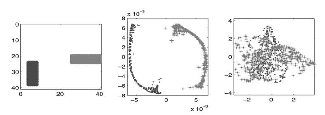
- Laplacian embedding better than PCA!
Laplacian embedding
Rough description
Given samples \(X_i, 1 \leq i \leq n\) in some metric space \((T, d)\), construct a graph \(G_n\) with Laplacian \(\Delta_n\)
Compute low-rank eigen decomposition (of smallest eigenfunctions!)
\[ \Delta_n = L_n \Lambda_n^{-1} L_n' \]
- “Embed” in \(\mathbb{R}^k\) for some user chosen rank \(k\):
\[ E^k_{n} = L_n \sqrt{\Lambda_n} \]
- At least locally, we hope (?)
\[ \|E^k_{n,i} - E^k_{n,j}\|_2 \approx d(X_i, X_j) \]
- A version of kernel PCA (with data-dependent kernel)
Why do we hope?
Suppose \(T\) is a Riemannian manifold \((M,g)\) that is densely sampled by the empirical measure \(\hat{\mathbb{P}}\)
Maybe \(\hat{\mathbb{P}}\) is close to Riemannian measure \(\mu\)
We hope \(L_n\) “look like” eigenfunctions of Laplacian associated to \((M,g)\)
\[ \Delta f = \lambda f, \qquad f \in L^2(\mu) \]
- Why do we care about \(x \mapsto (\lambda_i^{-1/2} f_i(x))_{1 \leq i \leq k} = E_k(x)\)?
A kernel of hope
- Consider
\[ {\cal H}_{\alpha} = \left\{f: f \in L^2(\mu): \langle f, \alpha(\Delta) f \rangle_{L^2(\mu)} < \infty\right\} \]
For appropriate choices of \(\alpha\), \({\cal H}_{\alpha}\) is an RKHS! (c.f. Sobolev embedding)
Set
\[ E_k(x) = \sum_{i=1}^k \alpha(\lambda_i)^{-1/2} f_i(x) \]
- And…
\[ \|E_k(x) - E_k(y)\|^2_{\mathbb{R}^k} \overset{k \to \infty}{\to} K_{\alpha}(x,y) \]
Fact: given any covariance kernel \(K:T \times T \to \mathbb{R}\), the map \(d(x,y) = \|K_x-K_y\|_{\cal H}\) is a (pseudo-metric) on \(T\)…
\(\implies\) if \(d^2(x,y) = \|K_{\alpha}(x) - K_{\alpha}(y)\|^2_{\cal H}\) then \(E_k\) are approximate embeddings…
This assumption implies our metric was Euclidean (in some asymptotic sense). Not all metrics are Euclidean…
Related differential geometry: Spectral geometry