Data Uncertainty

All fundamental combustion experimental data have uncertainties. The data uncertainties must be evaluated before using them in reaction model optimization or validation. The source of data uncertainties comes from statistical consistency, experimental techniques, post-processing of the data, among many other sources. In this section, we introduce a systematic framework to quantify the uncertainties for typical combustion experimental data.

Statistical consistency

One source of uncertainty is the statistical consistency. Over the past decades, the combustion properties of certain thermodynamic conditions have been measured multiple times, by various research groups using different experimental techniques. To this end, we carry out a statistical analysis using empirical function analysis and nonlinear least square procedure¹. The statistical scatter is calculated by the prediction confidence interval using

\[\begin{equation} \delta(\alpha) = t(1 - \frac{\alpha}{2}, n_{df}) \Big\{ \Big[\frac{\sum_{j=1}^n (y_{data, j} - \hat y_{fit,j})^2}{n_{df}} \Big] \Big[1 + \frac{1}{n} + \frac{(x - x_{mean})^2}{\sum_{j=1}^n (x - x_{mean})^2} \Big] \Big\}^{1/2} \end{equation}\]

The equation above calculates the $\alpha$ confidence interval, where $t$ is the Student-t distribution; $y_{fit}$ represents the prediction by the empirical functions; $y_{data}$ represents the laminar flame speed measurement $S_u^o$ or the normalized ignition delay measurement $\tau_{ign}[\text{Fuel}]^{-\alpha} [\text{O}_2]^{-\beta} [\text{Diluent}]^{-\gamma}$. The total number of data points is $n$ and the degree of freedom is $n$_$df$. $x$ represents the normalized equivalence ratio $\bar \phi$ or the normalized post-shock temperature $1000 \text{ K} / T_5$.

Laminar Flame Speed

For laminar flame speed, the rational function is used to express the variation of flame speed as a function of the normalized equivalence ratios $\bar \phi$.

\[\begin{equation} S_{u, calc}^o (\bar \phi) = \frac{P(\bar \phi)}{Q(\bar \phi)} = \frac{\sum_{i=0}^{n_p} p_{i} \bar \phi^{i}}{1 + \sum_{i=1}^{n_q} q_{i} \bar \phi^{i}} \end{equation}\]

where $P$, $Q$ are polynomials and $p_i$, $q_i$ are the associated coefficients. The orders of the polynomials $n_p$, $n_q$ are hyper-parameters to be determined through a convergence test on the fit. The normalized equivalence ratio $\bar \phi$ removes the asymmetric variation of flame speed with equivalence ratio $\phi$ between the fuel lean region ($\phi \in [0,1]$) and the fuel rich region ($\phi \in [1, \infty]$)¹.

\[\begin{equation} \bar \phi = \frac{\phi}{1 + \phi} \end{equation}\]

We demonstrate the analysis with the laminar flame speed of $i$-C₄H₈/air mixtures at unburnt gas temperature $T_u = 298$ K and pressure $p = 1$ atm as an example. The given condition has been measured by 7 research groups from 1998 to 2016. Davis and Law² conducted experiments for equivalence ratios $\phi=0.7-1.7$ using the counterflow twin-flame configuration and the stretch effect of the flame speed measurements was corrected using linear extrapolation. Kelly³ and Zhao et al.⁴ measured the flame speeds for equivalence ratios $\phi = 0.7-1.8$ using the outwardly propagating spherical flames in a double-chamber constant-pressure combustion bomb and applied a nonlinear regression approach to correct for the stretch effects. Park et al.⁵ used the counterflow twin-flame technique and obtained the stretch-free data using computationally-assisted nonlinear extrapolation. In a multi-university collaboration work, Zhou et al.⁶ provided data from three universities. Princeton University (PU) and Texas A&M University (TAMU) took the measurements using the spherical bombs, wheras CNRS-Université de Lorraine (CNRS) employed the heat flux method. TAMU data were obtained in a high-temperature, high-pressure, constant-volume bomb with nonlinear extrapolation. Princeton data were obtained in a cylindrical chamber with a concentric release chamber, followed by linear extrapolation to zero stretch.

Figure 1 plots all data discussed above. The red solid line represents the nominal fit of the data using the rational function. The two blue dash dot lines are the 95% confidence intervals, which gives a quantitative assessment of the statistical scatter of the data. The data in blue symbols (Davis and Law²) lie outside of the confidence interval for the fuel rich conditions. This is attributed to the linear extrapolation. This set of data is removed and the fitting is conducted iteratively until no outliers are observed or outliers cannot be explained by data interpretation. This analyses also helps to direct future experiments. For the flame speed of $i$-C₄H₈/air mixture, the fuel rich conditions exhibit smaller data scatter than the fuel lean conditions. The large scatter under the fuel lean condition are due to two sets of data, one from Princeton, and the other from TAMU: they differ for about $5-7$ cm/s and the reason for the discrepancy remains unclear according to the original paper⁶. Clearly, data under the fuel lean condition will be needed to further reduce the data ncertainty,

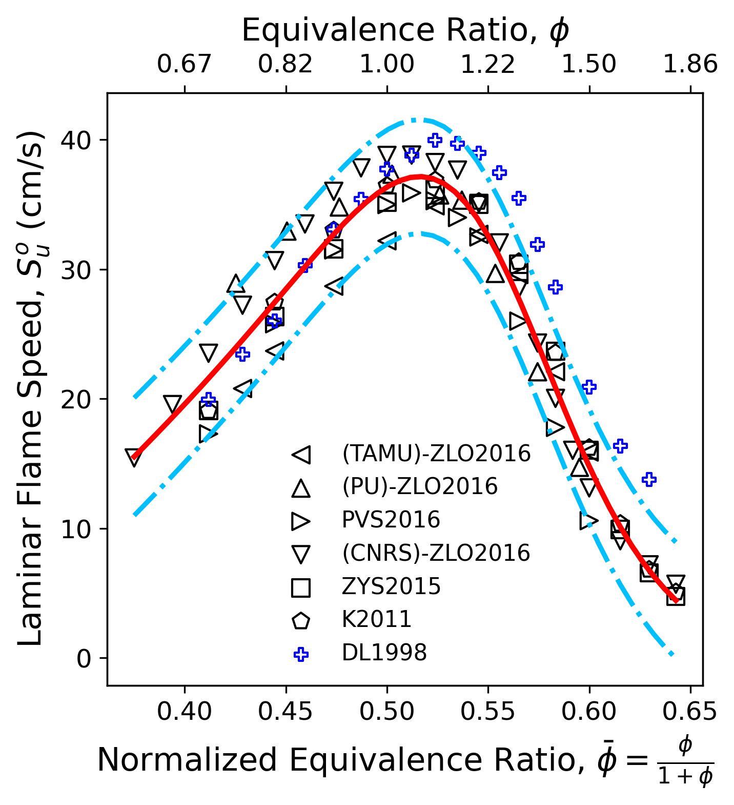
Figure 1 The statistical consistency analysis for laminar flame speed of iso-butene / air mixture at 298 K and 1 atm

For the data shown in Fig. 1, the calculated $2\sigma$ uncertainty is treated as the statistical consistency factor and used for model optimization; for data that are measured less than three times, we use 10% of the measured values to represent the statistical consistency. To factor in other effects, the flame speed uncertainty is lower bounded by 5% of the nominal values.

Ignition Delay Time

For ignition delay measurements, the experimental data are fitted by the widely used Lifshitz function, where $A, n, B, \alpha, \beta, \gamma$ are coefficients and [Fuel], [O₂] and [Diluent] represent the species concentration calculated by the ideal gas law.

\[\begin{equation} \tau_{ign, calc} (T) = A T^n \exp(\frac{B}{T_5}) [\text{Fuel}]^{\alpha} [\text{O}_2]^{\beta} [\text{Diluent}]^{\gamma} \end{equation}\]

Figure 2 collects ignition delay measurements for ethylene/oxygen mixtures diluted in argon from 1967 to 2021. Similarly, the red solid line represents the nominal fit using Lifshitz function, while the two dash dot lines are the 95% confidence intervals. Outlier data are again evaluated based on the experimental techniques used.

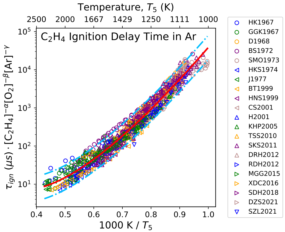
Figure 2 The statistical consistency analysis for ignition delay time of ethylene/oxygen/argon mixture at various temperature, pressure and compositions.

Generic effects

In laminar flame speed measurements, many aspects could contribute to the uncertainties, including hydrodynamic instabilities of spherical flames at elevated pressures; inappropriate flame stretch corrections in spherical flames and counterflow measurements; heat-loss through the walls or radiation which challenges the adiabatic assumptions. Woith all factors considered, the uncertainty in the currently available laminar flame speed measurements is at least 5%⁷. In our evaluation of flame speed uncertainty, we use 5% of the measured value as the lower bound for $2\sigma$ data uncertainty.

For shock tube measurements, impurity and temperature uncertainty contribute to data uncertainties. Computer experiments are used to quantify such effects,

• for the impurity effect, ignition delay is calculated using the reported mixture composition with and without H radical added to represent the impurity effect. The difference between the two calculated values are included in the uncertainty quantification. The amount of H radical is determined using a fitted Arrhenius expression⁸.

• for the temperature uncertainty, the given T₅ is perturbed by $\pm$1% in kinetic simulations, the difference was included in the uncertainty quantification.

The overall uncertainty factor of a target considers all the factors discussed above.

References

---