Monte Carlo Simulation

Monte Carlo sampling and computer experiments

Table of contents

1. Parameter sampling
   1. Sobol sequence
   2. Three sets of data samples
   3. Sample sizes
2. Computer experiments and computational cost
   1. Simulation details
   2. Computational cost
3. References

Parameter sampling

Sobol sequence

The dimensionality for FFCM-2 optimization is high (1052 parameters and 1192 targets). In such high-dimensional parameter space, the plain random sampling approach causes clusters and holes, as shown in Fig. 1, which reduces the statistical sample efficiencies. In the FFCM-2 effort, the Sobol sequence sampling is used to address this issue. The Sobol sequence is an example of quasi-random low-discrepancy sequences, which successively add new sample points to positions as far away as possible from existing ones to avoid clustering. The Sobol sequence thus yields a good coverage of the input parameter space, and has been demonstrated to have the best convergence properties. We used the Python library scipy.stats.qmc.Sobol to generate the Sobol sequences.

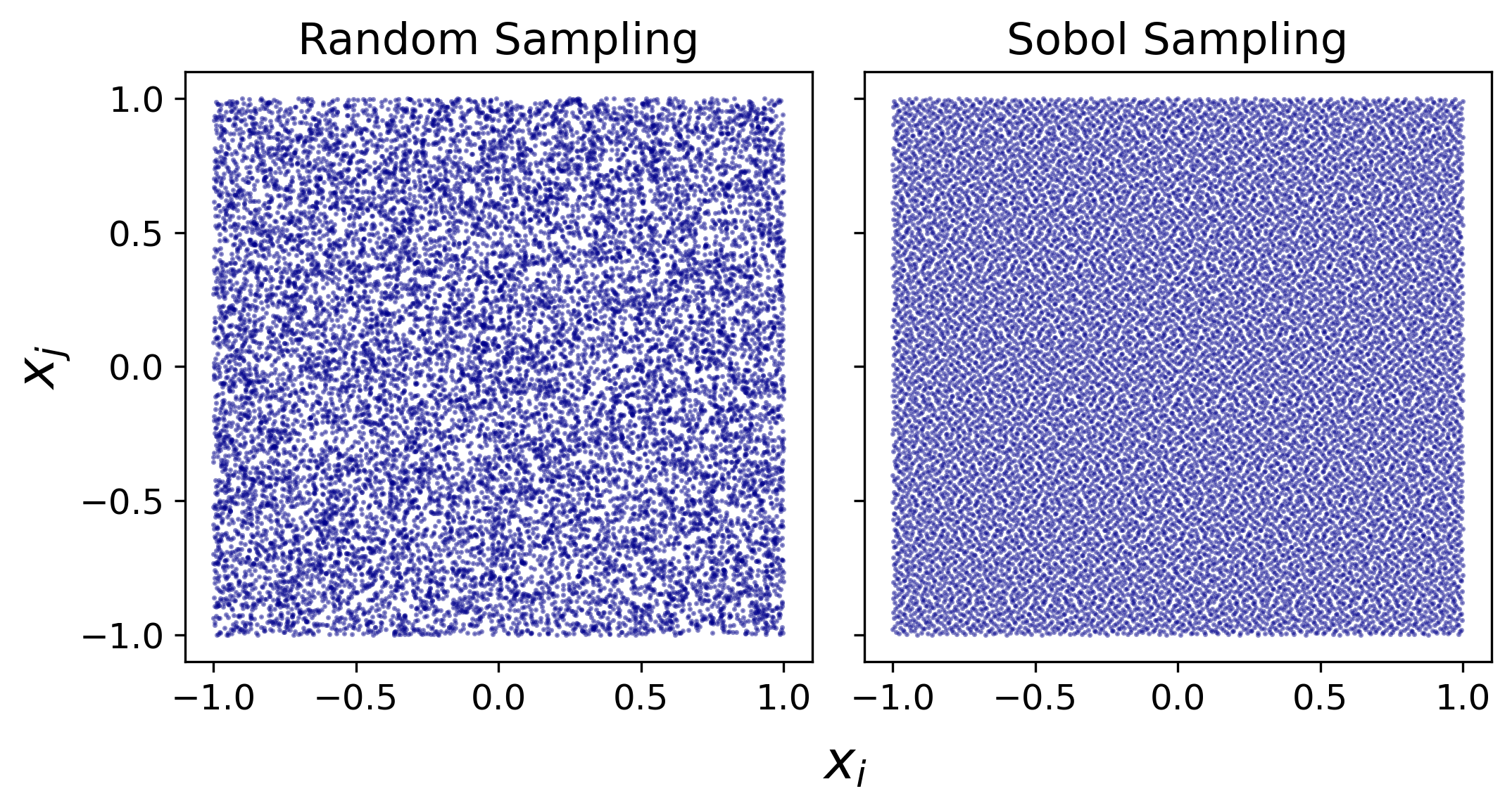
Figure 1 Projection of 32768 samples that are generated from a 1052-dimensional space within range $[-1,1]$ on two random dimensions. Left panel: random sampling that leads to clusters and holes; Right panel: Sobol sequence sampling that covers the space with low-discrepancy.

Three sets of data samples

The Sobol sequences are inherently uniform with respect to the sampled space and is thus inadequate because most samples would have been too far from the origin of the $N$-dimensional space. With the uniform Sobol samples, the NN response surfaces becomes under-trained especially around the center of the parameter space (the trial model). To this end, we transform the uniform Sobol sequences to multivariate normal distribution using the inverse of the cumulative distribution function (CDF) and truncate the normal distribution at physical bounds –1 and +1 to control the sample spaces within physical limits. The transformation function used is implemented in scipy.stats.truncnorm.ppf.

Additionally, we designed a sampling approach that highlights the need of accuracy around $\mathbf{x} = \mathbf{0}$ and yet considers the far edge of the parametric space as well. When transforming the uniform sequences to Gaussian, we consider three sub-spaces of the Gaussian samples parameterized by the standard deviation. Set 1 has a standard deviation of 0.1 in $\textbf{x}$; Sets 2 and 3 have standard deviations of 0.3 and 0.5, respectively. Set 3 has twice more sample points assigned to it than Sets 1 and 3. Together, the three sets form the complete sample set, as shown in Fig. 2.

Figure 2 Two-dimensional projections of Sobol sampling following a truncated inverse cumulative Gaussian distribution. The final set of samples comprises of three Gaussian-weighted subsets with standard deviations of 0.1, 0.3, and 0.5 in the $\mathbf{x}$ value for Sets 1, 2 and 3, respectively. Lower right panel: histograms of the sample counts of each sub set, as a function of root-mean squares of $\mathbf{x}$ (representing the distance of the sample to the origin). Note that Set 3 has twice more sample points than Sets 1 and 2.

Sample sizes

For FFCM-2 with 1052 parameters, we found a combined data sample size of 10,000 to be appropriate for the laminar flame speed and 40,000 to be appropriate for logarithms of the ignition delay and species concentration. The choice for the sample size takes into consideration the computational cost, effect sparsity, and the performance of the resulting NN-RS. The samples were partitioned as follows: 80% of data were randomly selected for NN training; 10% were used for validating the hyper-parameter choices; the remaining 10% were used for NN-RS validation.

Computer experiments and computational cost

In the current work, all kinetic simulations were carried out in the Cantera software with a Python interface¹.

Simulation details

For shock tube and flow reactor experiments, we used the Zero-Dimensional Reactor Network to solve the initial value problem. The ignition delay times was solved using the adiabatic, constant-volume assumption unless stated otherwise; and the computed ignition delay was determined in a manner consistent with the experiment. The shock tube speciation measurements and the flow reactor experiments are simulated using adiabatic, constant-pressure assumption; The One-dimensional Reacting Flow module was used to solve for the laminar flame speed, with multi-component transport and thermal diffusion. Each solved flame was converged with GRAD and CURV below 0.02, using at least 400 mesh grids.

Computational cost

All the computations were performed on Sherlock, the Stanford Research Computing Center (SRCC). On the computing clusters, it takes about one second to compute the shock tube ignition delay or species time-histories. For the laminar flame speed, the trial model was used to obtain the converged flame object. The solution is then used as a restart file for the subsequent flame calculations. On average, each flame calculation takes 15-30 seconds with restart file. A simple NN-RS for ignition delay time may require 40,000 training samples, which translates to about 12 CPU hours; for flame speed requiring 10,000 training samples, around 60 CPU hours is needed. Training the NN-RS takes around five to seven minutes each.

Note that the major computational cost lies in the Monte Carlo simulation for generating training samples in the NN-MUM-PCE framework. Once the response surfaces are generated, the optimization run takes about two minutes for all targets.

References

---