Neural Networks
Neural network response surfaces
Table of contents
- Neural network architecture
- NN training and hyper-parameter tuning
- Evaluation metrics
- Adaptive NN training
- Generalized NN with thermodynamic conditions as input
- References
FFCM-2 is a substantially high-dimensional optimization problem. The conventional approach of using polynomials as reponse surfaces with 20-30 truncated rate parameters leads to significant truncation errors. Also, training each target from scratch is computationally expensive and thus limits the scalability of polynomials to large size targets. To address these issues, we used neural networks as response surfaces for FFCM-2 development1.
Neural network architecture
Simple NN-RS
Figure 1 shows the architecture of a simple, single-condition neural network response surface. Given the thermodynamic conditions of a certain combustion fundamental property, the normalized rate parameters are mapped to the computed data.
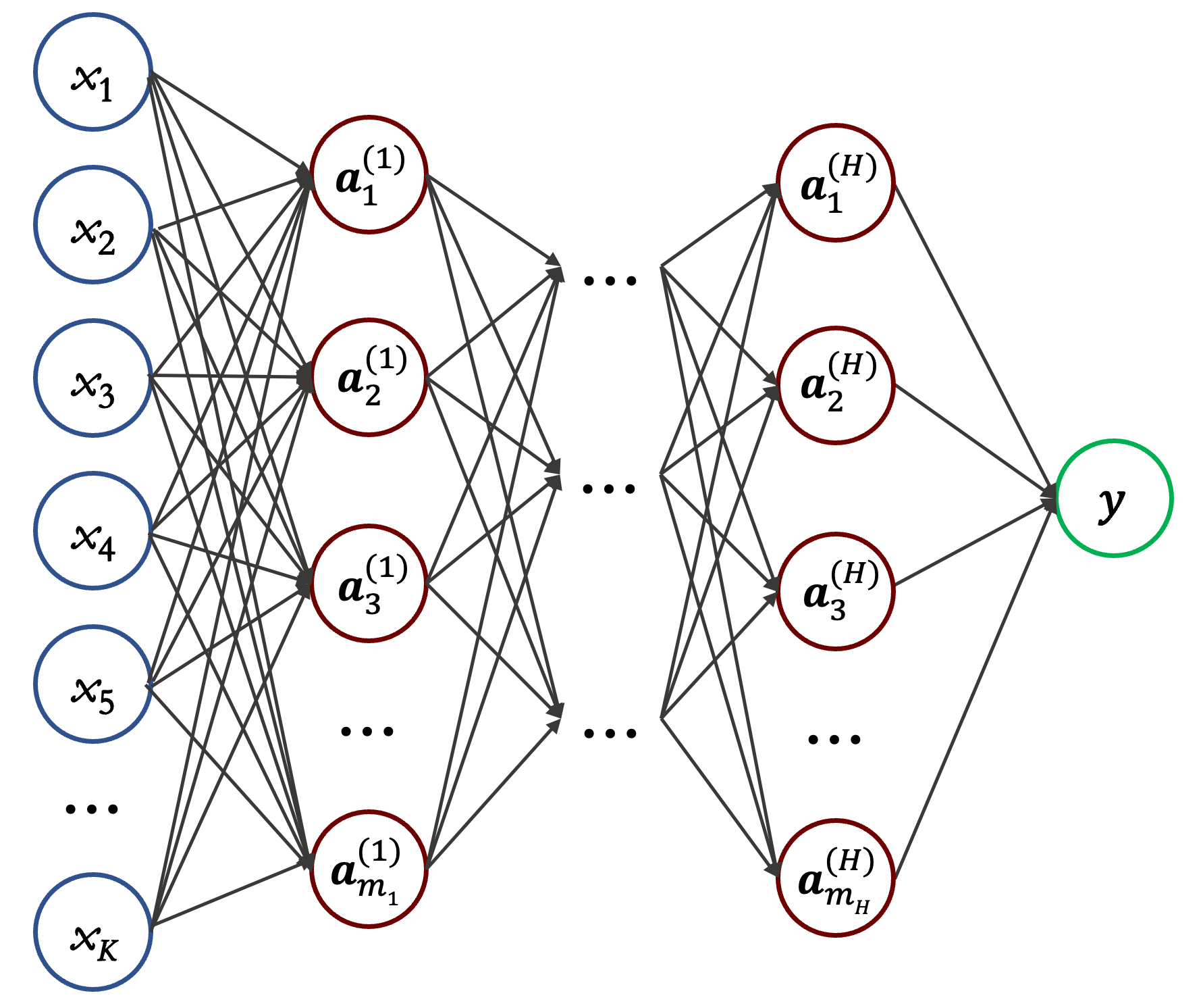
Figure 1 The archictecture of the simple, single-condition neural network response surface. The left most (blue) layer is the input layer of $K$ input variables (normalized rate parameters); the right most (green) layer is the single-node output layer; the layers in between (red) are the hidden layers numbered as $1,2,...,H$, with $m_1,m_2,...,m_H$ hidden nodes, respectively, for each layer.
Listed below are the mathematical equations for a one-hidden layer NN-RS, where $\mathbf{x} \in \mathbb{R}^{K}$ is the input normalized reaction rate parameters, $K$ is the number of active parameters. $m_1$ defines the number of hidden nodes in the first hidden layer, and it is a hyper-parameter to be determined during the neural network training. $\mathbf{W_1, W_2, b_1}, b_2$ are the fitting coefficients to be determined. Note that this simple NN-RS is designed for training response surface of one target. For the targets considerd in current work, $m_1 = 16$ is found to be sufficient, which aligns with the fact that most targets are sensitive to around 20 rate parameters.
\[\begin{align} y &= \mathbf{W_2} \mathbf{a} + b_2, \mathbf{W_2} \in \mathbb{R}^{1 \times m_1}, b_2 \in \mathbb{R} \\ \mathbf{a} &= \phi(\mathbf{z})\\ \mathbf{z} &= \mathbf{W_1} \mathbf{x} + \mathbf{b_1}, \mathbf{W_1} \in \mathbb{R}^{m_1 \times n}, \mathbf{b_1} \in \mathbb{R}^{m_1}\\ \end{align}\]Generalized NN-RS
In large-scale optimziation, many targets have thermodynamic conditions that are heavily correlated. To this end, we proposed a generalized NN-RS that takes as input the thermodynamic conditions of an array of targets. It is deeper, with more training parameters and needs more training samples. The benefits is obvious: the total amounts of training samples are significantly reduced for all targets.
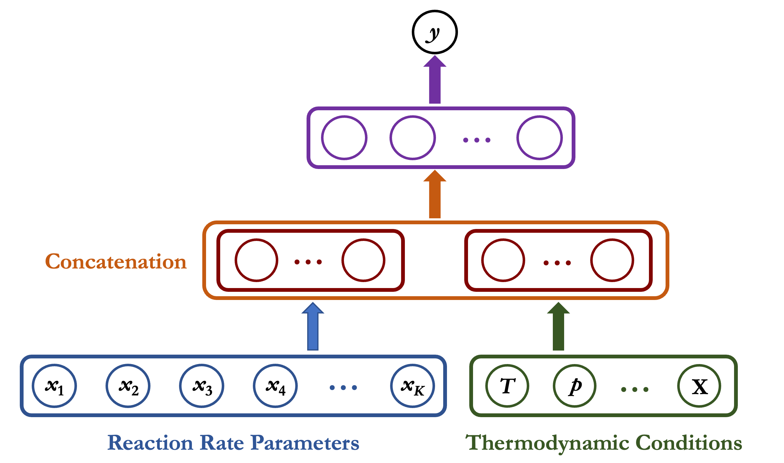
Figure 2 A generalized NN-RS architecture that incorporates the thermodynamic conditions as input. For the bottom layer, the normalized reaction rate parameters $\mathbf{x}$ (in blue) and thermodynamic conditions (eg., temperature $T$, pressure $p$ and mixture composition $\mathbf{X}$) (in green) are processed as two separate sets of coefficients. In the second layer, the two processed vectors (red) are concatenated (orange) and passed through the third layer (purple) to predict the combustion responses.
NN training and hyper-parameter tuning
For all NN training, we used 1024 as the training batch size to train 5000 epochs, using as the loss function the mean squared error loss (MSELoss) implemented in the PyTorch library. After every 10 epochs, we evaluate performance against the validation set and keep track of the best-performing NN-RS. After 5000 epochs, the best performer was chosen as the final NN-RS.
The hyper-parameters describe the neural network structures (e.g., number of hidden nodes and hidden layers) or determine the neural network optimization (e.g., learning rates). The performance of NN-RS depends heavily on the choice of the hyper-parameters during training2. The most important hyper-parameters for the neural network optimization are the learning rate and the weight decay parameter. An appropriate learning rate is crucial because too high of a learning rate leads to instability and difficulties in finding optimal solution, and too low of a learning rate becomes computationally expensive. Obtaining an optimal learning rate requires experimentation. We adopted an initial learning rate from the learning rate finder3 and then during training, successively reduced this rate to achieve convergence.
We found an initial learning rate of 0.03 to be roughly optimal. We used the ReduceOnPlateau learning rate scheduler to reduce the rate by a factor of two when the performance improvement on the test and validation data becomes stagnant after every 200 training epochs.
The weight decay is an important parameter that controls underfitting and overfitting of the neural network. When the training loss plateaus at a value much lower than the validation loss, we increase the weight decay value to reduce the potential of overfitting; when training loss and validation loss plateaus together at higher values, we reduce the weight decay parameter to allow for more flexibility. We used the Adam optimizer and found $10^{-4}-10^{-3}$ to be the optimal weight decay.
Evaluation metrics
The selected final NN-RS during training is subject to additional performance test before being used in optimization. To this end, we calculated the relative errors on the test data. Specifically, for the $m^{th}$ data point in the test set, we calculate
\[\begin{equation} e_m = \frac{|y_{m,nn} - y_{m,calc}|}{y_{m,calc}} \end{equation}\]where $y_{m, nn}$ and $y_{m, calc}$ are predicted by an NN-RS and calculated from computer experiment, respectively. Note that although we fit the NN-RS using logarithm of the response values of the ignition delay times and species concentrations, the performance is evaluated based on the original calculated value. This provides a more stringent requirement on the performance of NN-RS.
The overall performance of NN-RS is evaluated by the mean relative error ($\varepsilon_{\rm{mean}}$) and 95-percentile relative error ($\varepsilon_{95\%}$) as the key evaluation metrics, as listed in the table below, because they are more indicative of the relevant parameter space away from sample outliers than the maximum relative error ($\varepsilon_{\rm{max}}$). The requirements are most stringent near the center of the parameter space (i.e., Set 1 with $\sigma = 0.1$), and are more relaxed farther from the center (i.e., Set 2 with $\sigma = 0.3$ and Set 3 with $\sigma = 0.5$).
| Test set | Mean error ($\varepsilon_{\rm{mean}}$) | 95-percentile error ($\varepsilon_{95\%}$) |
|---|---|---|
| Set 1 ($\sigma = 0.1$) | 1% | 2% |
| Set 2 ($\sigma = 0.3$) | 2% | 5% |
| Set 3 ($\sigma = 0.5$) | 3% | 10% |
Adaptive NN training
One key advantage that neural network brings is the adaptiveness of the trained NN-RS, which can effectively reduce the training samples needed for large size optimization. Three case studies are discussed to illustrate the point.
Case I: Adapt to related thermodynamic conditions
Targets with related thermodynamic conditions have similar reaction kinetics, and thus a neural network trained can be adapted to related conditions with significantly reduced training samples. Consider a trained NN-RS for the ignition delay of a stoichiometric CH4-O2-77.5% CO2 mixture at the nominal $p_5 = 32.8$ atm and $T_5=1421$ K condition (center star). To adapt to related conditions that vary $T_5$ and $p_5$ as illustrated in Fig. 3, we initialize the new NN-RS with the trained NN-RS (center star). Figure 4 shows that adaptively trained NN-RS can reduce the additional training samples to as much as 1% of the original sample size (case $A$).
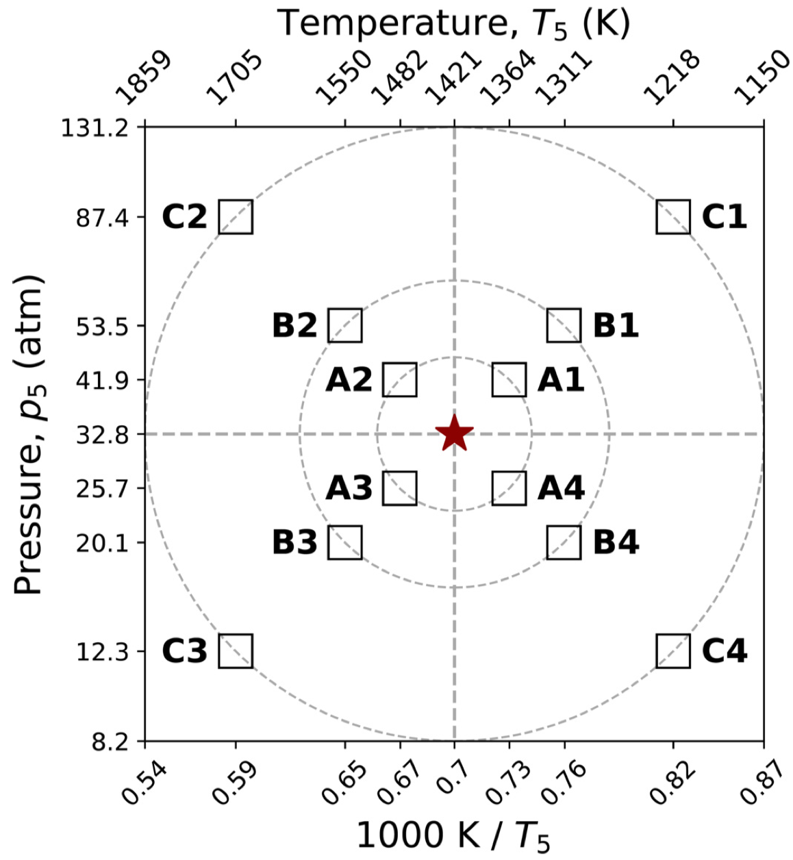
Figure 3 Selected thermodynamic conditions for adaptive training using the NN already trained for the ignition delay of a stoichiometric CH4-O2-77.5% CO2 mixture at the nominal p5 and T5 condition marked by the center star. Three sets of new conditions are tested with each set containing the variations of both p5 and T5 . The set closest to the nominal condition is denoted as set A; the intermediate set is B; the furthest set is C, which extends p5 from 12.3 atm to 87.4 atm, and of T5 from 1,218 K to 1,705 K.
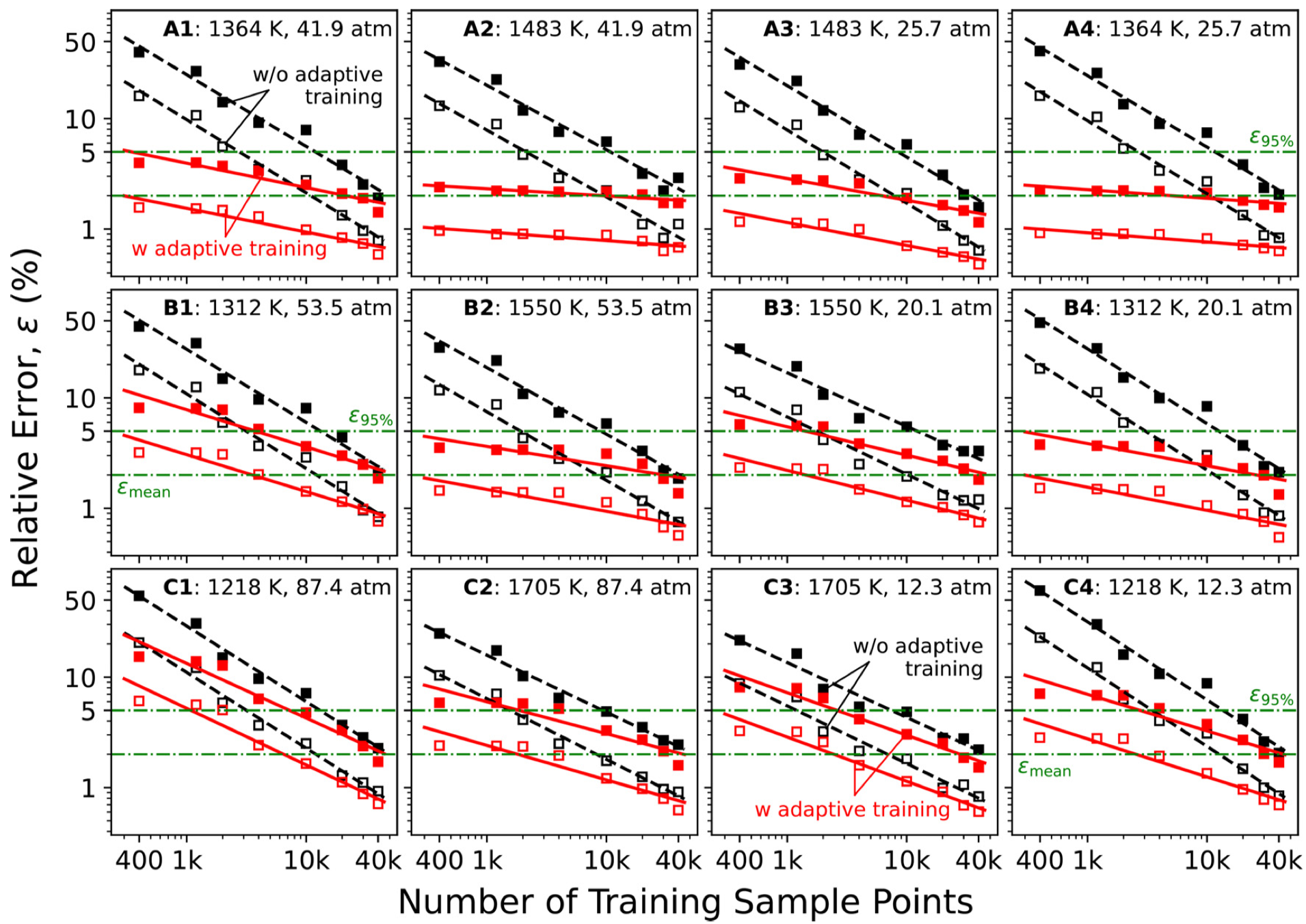
Figure 4 Comparison of mean (open symbols) and 95-percentile (filled symbols) errors as a function of the number of samples used for NN training, comparing adaptive training (solid lines) and without adaptive training (dashed lines) for the three sets of conditions $(A_i$: top panels, $B_i$: middle panels, and $C_i$: bottom panels, for $i=1,...,4)$ shown in Fig. 3. The horizontal dashed-dotted-dashed lines indicate the mean and 90-percentile error tolerance levels. Tests use Set 2 of the data sample with 2,000 sample points. Lines are drawn to guide the eyes.
Case II: Adapt to augmented input parameters
Reaction model optimization may often need to add missing reactions or splits one or more rate parameters to augment the input dimension. The NN-RS, in this case, can adapt to learn the coefficients for the new weights, while keeping the knowledge of the remaining physics. In our recent work1, we studied the response surface for ignition delay time of stoichiometric C2H6/O2 mixtures diluted in 91% argon with T5 = 1434 K and p5 = 7.56 atm. In the base case, the reaction
\[\begin{equation} \text{C}_2\text{H}_4 + \text{H (+M)} \rightleftharpoons \text{C}_2\text{H}_5 \text{ (+M)} \end{equation}\]was treated using only one independent input parameter. Suppose that the Chaperon efficiencies of Ar, N2 and H2O must be treated separately in optimization against the ignition delay (in argon) and laminar flame speed (in N2, where M = H2O exerts a notable impact on the flame speed). Splitting M into M = Ar, M = H2O, M = N2 and all other species forms an extended NN, which needed only 4,000 samples or 10% of those in the base case for its training, as shown in a recent work1.
Case III: Adapt to updates of the trial rate parameters
The trial rate parameters need to be updated when new reaction rate theories or experimental measurements are available. In this case, we consider reaction model updates focusing on the iso-butene sub-model. A total of 13 iso-butene related reactions were updated from an earlier FFCM-2 trial model, including the H-abstraction by O2 of iso-butene by considering recent theoretical calculation4 and low-temperature rate measurements5.
\[\begin{equation} i\text{-C}_4\text{H}_8 + \text{O}_2 \rightleftharpoons i\text{-C}_4\text{H}_7 + \text{HO}_2 \end{equation}\]We used the ignition delay time of 2% iso-butene - 12% O2 diluted in Ar at $T_5 = 1556$ K and $p_5=1.7$ atm as the test case. Adaptive NN training required 12000 training samples (about 30% of the original training data) to achieve the same accuracy of the base case NN. Although the iso-butene sub-model has been changed significantly, the reduced number of training samples indicate useful knowledge transfer from the base-case NN to the adapted NN, which comes from key reactions beyond the iso-butene submodel, e.g.,
\[\begin{align} \text{H + O}_2 &\rightleftharpoons \text{O + OH}\\ \text{CH}_3\text{ + HO}_2 &\rightleftharpoons \text{CH}_3\text{O + OH} \end{align}\]Generalized NN with thermodynamic conditions as input
We provide an example of the generalized NN-RS trained for laminar flame speeds of CH3OH/air mixtures. Figure 5 shows that response surfaces over a wide range of initial temperature, pressure and equivalence ratios are covered by one generalized neural network using 60,000 training samples. It also shows the projection of the generalized NN-RS on a low-dimensional space.

Figure 5 Generalized NN-RS for laminar flame speeds of CH3OH/air mixtures at temperature 298 - 450 K, pressure 0.5 - 10 bar and equivalence ratio 0.6 - 1.8, with active parameters K = 1052, expressed as $y_{S_u^o} (\mathbf{x}, T_0, p, \phi)$. The figure above shows the projection of the generalized NN-RS.
References
-
Zhang, Y., Dong, W., Vandewalle, L. A., Xu, R., Smith, G. P., & Wang, H. (2023). Neural network approach to response surface development for reaction model optimization and uncertainty minimization. Combustion and Flame, 251, 112679. ↩ ↩2 ↩3
-
Smith, L. N. (2018). A disciplined approach to neural network hyper-parameters: Part 1–learning rate, batch size, momentum, and weight decay. arXiv preprint arXiv:1803.09820. ↩
-
Smith, L. N. (2017). Cyclical learning rates for training neural networks. In 2017 IEEE winter conference on applications of computer vision (WACV) (pp. 464-472). IEEE. ↩
-
C. W. Zhou, J. M. Simmie, K. P. Somers, C. F. Goldsmith, H. J. Curran, Chemical kinetics of hydrogen atom abstraction from allylic sites by $^3$O$_2$; implications for combustion modeling and simulation, J. Phys. Chem. A 121 (2017) 1890–1899 ↩
-
T. Ingham, R. Walker, R. Woolford, Kinetic parameters for the initiation reaction RH + O$_2$ = R + HO$_2$, Symp. (Int.) Combust. 25 (1994) 767–774 ↩