Chapter 8
Recurrent Backpropagation: Attractor network models of semantic
and lexical processing
Recurrent back-propagation networks came into use shortly after the development
of the back-propagation algorithm was first developed, and there are many variants
of such networks. Williams and Zipser (1995) provide a thorough review of the
recurrent back-propagation computational framework. Here we descibe a particular
variant, used extensively in PDP models the effects of brain injury on lexical and
semantic processing (Plaut and Shallice, 1993; Plaut et al., 1996; Rogers
et al., 2004; Dilkina et al., 2008).
8.1 BACKGROUND
A major source of motivation for the use of recurrent backpropagation networks in
this area is the intuition that they may provide a way of understanding the
pattern of degraded performance seen in patients with neuropsychological
deficits. Such patients make a range of very striking errors. For example, some
patients with severe reading impairments make what are called semantic
errors – misreading APRICOT as PEACH or DAFFODIL as TULIP. Other
patients, when redrawing pictures they saw only a few minutes ago, will
sometimes put two extra legs on a duck, or draw human-like ears on an
elephant.
In explaining these kinds of errors, it has been tempting to think of the patient as
having settled into the wrong basin of attraction in a semantic attractor
network. For cases where the patient reads ‘PEACH’ instead of ‘APRICOT’,
the idea is that there are two attractor states that are ‘near’ each other
in a semantic space. A distortion, either of the state space itself, or of the
mapping into that space, can result in an input that previously settled to
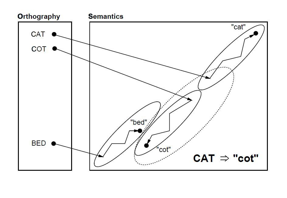
one attractor state settling into the neighboring attractor. Interestingly,
patients who make these sorts of semantic errors also make visual errors, such
as misreading ‘cat’ as ‘cot’, or even what are called ‘visual-then-semantic’
errors, mis-reading ‘sympathy’ as ‘orchestra’. All three of these types of errors
have been captured using PDP models that rely on the effects of damage in
networks containing learned semantic attractors (Plaut and Shallice, 1993).
Figure 8.1 from Plaut and Shallice (1993) illustrates how both semantic and
visual errors can occur as a result of damage to an attractor network that
has learned to map from orthography (a representation of the spelling of a
word) to semantics (a represenation of the word’s meaning), taking printed
words and mapping them to basins of attraction within a recurrent semantic
network.
The use of networks with learned semantic attractors has an extensive history in
work addressing semantic and lexical deficits, building from the work of Plaut and
Shallice (1993) and other early work (Farah and McClelland, 1991; Lambon Ralph
et al., 2001). Here we focus on a somewhat more recent model introduced
to address a progressive neuropsychological condition known as semantic
dementia by Rogers et al. (2004). In this model, the ‘semantic’ representation
of an item is treated as an attractor state over an population of neurons
thought to be located in a region known as the ‘temporal pole’ or anterior
temporal lobe. The neurons in this integrative layer receive input from, and
project back to, a number of different brain regions, each representing a
different type of information about an item, including what it looks like, how it
moves, what it sounds like, the sound of its name, the spelling of the word
for it, etc. The architecture of the model is sketched in Figure 8.2 (top).
Input coming to any one of the visible layers can be used to activate the
remaining kinds of information, via the bi-directional connections among
the visible layers and the integrative layer and the recurrent connections
among the units in the integrative layer. According to the theory behind the
model, progressive damage to the neurons in the integrative layer and/or to
the connections coming into and out of this integrative layer underlies the
progressive deterioration of semantic and abilities in semantic dementia patients
(?).
8.2 THE RBP PROGRAM
In the version of recurrent back propagation that we consider here, activations of
units are thought of as being updated continuously over some number of time
intervals. The network is generally set to an initial state (corresponding to time 0), in
which some units are clamped to specific values by external inputs, while others are
initialized to a default starting value. Processing then proceeds in what is
viewed conceptually as a continuous process for the specified number of time
intervals. At any point along the way, target patterns can be provided for
some of the pools of units in the network. Typically, these networks are
trained to settle to a single final state, which is represented by a target to be
matched over a subset of the pools in the network, over the last few time
intervals.
At the end of the forward activation process, error signals are “back propagated
through time” to calculate delta terms for all units in the network across the entire
time span of the settling process. A feature of recurrent back-propagation is that the
same pool of units can have both external inputs (usually provided over the first few
time intervals) and targets (usually specified for the last few intervals). These
networks are generally thought of as settling to attractor states, in which there is a
pattern of activation over several different output pools. In this case, the target
pattern for one of these pools might also be provided as the input. This captures the
idea that I could access all aspects of my concept of, for example, a clock, either
from seeing a clock, hearing a clock tick, hearing or reading the word clock,
etc.
One application of these ideas is in the semantic network model of Rogers
et al. (2004). A schematic replica of this model is shown in Figure 8.2 (top). There
are three sets of visible units, corresponding to the name of the object, other
verbal information about the object, and the visual appearance of the object.
Whichever pattern is provided as the input, the task of the network is to settle to
the complete pattern, specifying the name, the other verbal information
about the object, and the visual percept. Thus the model performs pattern
completion, much like, for example, the Jets-and-Sharks iac model from
Chapter 2. A big difference is that the Rogers et al. (2004) model uses
learned distributed representations rather than instance units for each known
concept.
8.2.1 Time intervals, and the partitioning of intervals into ticks
The actual computer simulation model, called rbp, treats time, as other networks do,
as a sequence of discrete steps spanning some number of cannonical time intervals.
The number of such intervals is represented by the variable nintervals. In rbp, the
discrete time steps, called ticks, can slice the whole span of time very finely or
very coursely, depending on the value of a parameter called dt. The number
of ticks per interval is 1∕dt, and the total number of ticks of processing is
equal to nintervals∕dt. The number of states of the network is one larger
than the number of ticks; there is an initial state, at time 0, and a state
at the end of each tick — so that the state at the end of tic 1 is state 1,
etc.
8.2.2 Visualizing the state space of an rbp network
To understand the recurrent backpropagation network, it is useful to visualize the
states of all of the units in the network laid out on a series of planes, with one plane
per state (Figure 8.2). Within each plane all of the pools of units in the network are
represented. Projections are thought of as going forward from one plane to the next.
Thus if pool(3) of a network receives a projection from pool(2), we can visualize
nticks separate copies of this projection, one to the plane for state 1 from
the plane for state 0, one to the plan for state 2 from the plan for state 2,
etc.
8.2.3 Forward propagation of activation.
Processing begins after the states of all of the units have been initialized to their
starting values for state 0. Actually, both the activations of units, and their net
inputs, must be initialized. The net inputs are set to values that correspond to the
activation (by using the inverse logistic function to calculate the starting net input
from the starting activation). For cases where the unit is clamped at 0 or 1, the
starting net input is based on the correct inverse logistic value for 2.0e-8 and
1-(2.0e-8). [CHECK]
After the net inputs and activations have been established for state 0, the net
inputs are calculated for state 1. The resulting net input value is essentially a running
average, combining what we will call the newnet, based on the activations at the
previous tick with the old value of the net input:
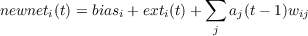
 Note that if dt = 1 (the largest allowable value), the net input is not time averaged,
and net(t) simply equals newnet(t).
Note that if dt = 1 (the largest allowable value), the net input is not time averaged,
and net(t) simply equals newnet(t).
After net inputs for state t have been computed, activation values for state t are
then computed based on each unit’s net input for state t. A variant on this
procedure (not available in the rbp simulator) involves using the newnet to
calculate a newact value, and then time averaging is then applied on the
activations:

Time-averaging the net inputs is preferred because net input approximates a neuron’s
potential while activation approximates its firing rate, and it is generally thought
that it is the potential that is subject to time averaging (‘temporal summation’).
Also, time-averaging the net input allows activation states to change quickly if the
weights are large. The dynamics seems more damped when time-averaging is applied
to the activations.
Once activation values have been computed, error measures and delta terms
(called dEdnet) are calculated, if a target has been specified for the given state of the
unit. The error is thought of as spread out over the ticks that make up each interval
over which the target is applied, and so the magnitude of the error at each
time step is scaled by the size of the time step. Either sum squared error
(sse) or cross entropy error (cee) can be used as the error measure whose
derivative drives learning. In either case, we compute both measures of error,
since this is fast and easy. The sse for a given unit at a given time step
is

where tgti(t) is the externally supplied target at tick t. The cce for a given unit at a
given time step is

In the forward pass we also calculate a quantity we will here call the ‘direct’ dEdnet
for each time step. This is that portion of the partial derivative of the error with
respect to the net input of the unit that is directly determined by the presence of a
target for the unit at time step t. If squared error is used, the direct dEdnet is given
by
 Note that the direct dEdnet will eventually be scaled by dt, but this is applied during
the backward pass as discussed below. Of course if there is no target the
directdEdneti(t) is 0.
Note that the direct dEdnet will eventually be scaled by dt, but this is applied during
the backward pass as discussed below. Of course if there is no target the
directdEdneti(t) is 0.
If cross-entropy error is used instead, we have the following simpler expression,
due to the cancellation of part of the gradient of the activation function with part of
the derivative of the cross entropy error:
 The
process of calculating net inputs, activations, the two error measures, and the direct
dEdnet takes place in the forward processing pass. This process continues until these
quantities have been computed for the final time step.
The
process of calculating net inputs, activations, the two error measures, and the direct
dEdnet takes place in the forward processing pass. This process continues until these
quantities have been computed for the final time step.
The overall error measure for a specific unit is summed over all ticks for which a
target is specified:
 This is done separately for the sse and the cce measures.
The activations of each unit in each tick are kept in an array called the activation
history. Each pool of units keeps its own activation history array, which has
dimensions [nticks+1, nunits]
8.2.4 Backward propagation of error
We are now ready for the backward propagation of the dEdnet values. We can think
of the dEdnet values as being time averaged in the backwards pass, just as the net
inputs are in the forward pass. Each state propagates back to the preceding state,
both through the time averaging and by back-propagation through the weights, from
later states to earlier states:
 where
where
 The
subscript k in the summation above indexes the units that receive connections from
unit i. Note that state 0 is thought of as immutable, so deltas need not be calculated
for that state. Note also that for the last state (the state whose index is nticks + 1),
there is no future to inherit error derivatives from, so in that case we have simply
have
The
subscript k in the summation above indexes the units that receive connections from
unit i. Note that state 0 is thought of as immutable, so deltas need not be calculated
for that state. Note also that for the last state (the state whose index is nticks + 1),
there is no future to inherit error derivatives from, so in that case we have simply
have
 For the backward pass calculation, t starts at the next-to-last state (whose
index is nticks) and runs backward to t = 1; however, for units and ticks
where the external input is hard clamped, the value of dEdnet is kept at
0.
For the backward pass calculation, t starts at the next-to-last state (whose
index is nticks) and runs backward to t = 1; however, for units and ticks
where the external input is hard clamped, the value of dEdnet is kept at
0.
All of the dEdneti(t) values are maintained in an array called dEdnethistory. As
with the activations, there is a separate dEdnet history for each pool of units, which
like the activation history array, has dimensions [nticks+1,nunits]. (In practice, the
values we are calling directdEdnet scaled by dt and placed in this history array on
the forward pass, and the contents of that array is thus simply incremented during
the backward pass).
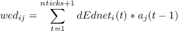
8.2.5 Calculating the weight error derivatives
After the forward pass and the backward pass, we are ready to calculate the
weight error derivatives arising from this entire episode of processing in the
network. This calculation is very simple. For each connection weight, we simply
add together the weight error derivative associated with each processing
tick. The weight error derivative for each tick is just the product of the
activation of the sending unit from the time step on the input side of the tick
times the dEdnet value of the receiving unit on the receiving side of the
tick:
8.2.6 Updating the weights.
Once we have the weight error derivatives, we proceed exactly as we do in the back
propagation algorithm as implemented in the bp program. As in standard back
propagation, we can update the weights once per pattern, or once per N patterns,
or once per epoch. Patterns may be presented in sequential, or permuted
order, again as in the bp program. Momentum and weight decay can also be
applied.
8.3 Using the rbp program with the rogers network
Training and testing in rbp work much the same as in other networks. The rogers
network has been set up in advance for you, and so you can launch the program to
run the rogers example by simply typing rogers at the MATLAB commmand
prompt while in the rbp directory. See Figure 8.3 for the screen layout of this
network.
During testing, the display can be updated (and the state of the network can be
logged) at several different granularities: At the tick level, the interval level, and
the pattern level. When tick level or interval level is specified, state 0 is
shown first, followed by the state at the end of the first tick or interval,
until the end of the final tick is reached. The template for the rogers model,
rogers.m, also displays the target (if any) associated with the state, below
the activations of each pool of units in the network. With updating at the
pattern level, the state is updated only once at the end of processing each
pattern.
Back propagation of error occurs only during training, although during
training the display update options are limited to the pattern and the epoch
level. The user can log activations forward and deltas back at the tick level
via the set write options button in the train options panel (select backtick
for ‘frequency’ of logging). Otherwise logging only occurs in the forward
direction.
8.3.1 rbp fast training mode.
A great deal of computing is required to process each pattern, and thus it takes quite
a long time to run one epoch in the rbp program. To ameliorate this problem, we
have implemented the pattern processing steps (forward pass, backward pass, and
computing the weight error derivatives) within a ‘mex’ file (essentially, efficient C
code that iterfaces with Matlab data formats and structures).Fast mode is
approximately 20 times faster than the regular mode. To turn on the fast mode for
network training, click the ’fast’ option in the train window. This option can
also be set by typing the following command on the MATLAB command
prompt:
runprocess(’process’,’train’,’granularity’,’epoch’,’count’,1,’fastrun’,1);
There are some limitations in executing fast mode of training.In this mode,
network output logs can only be written at epoch level. Any smaller output frequency
if specified, will be ignored.When running with fast code in gui mode, network viewer
will only be updated at epoch level.Smaller granularity of display update is disabled
to speed up processing.
There is a known issue with running this on linux OS.MATLAB processes running
fast version appear to be consuming a lot of system memory. This memory
management issue has not been observed on windows. We are currently
investigating this and will be updating the documentation as soon as we find a
fix.
8.3.2 Training and Lesioning with the rogers network
As provided the training pattern file used with the rogers network, (features.pat)
contains 144 patterns. There are 48 different objects (eight each from six categories),
with three training patterns for each. One provides external input to the name units,
one to the verbal descriptor units (one large pool consisting of ‘perceptual’,
‘functional’ and ‘encyclopedic’ descriptors) and one provides input to the
visual features units. In all three cases, targets are specified for all three
visible pools. Each of the three visible pools is therefore an ‘inout’ pool.
The network is set up to use Cross-Entropy error. If cross entropy error
is not used, the network tends to fail to learn to activate all output units
correctly. With cross-entropy error, this problem is avoided, and learning is quite
robust.
If one wanted to simulate effects of damage to connections in the rogers network,
the best approach would be to apply a mask to the weights in particular projections.
For example, to lesion (i.e. zero out) weights in net.pool(4).proj(3) with r receivers
and s senders, with a lesion probability of x:
- First save your complete set of learned weights using the save weights
command.
- Type the following to find the number of receivers r and senders s:
[r s] = size(net.pool(4).proj(3).weight);
- Then create a mask of 0’s and 1’s to specify which weights to destroy (0) and
which to keep (1):
mask = ceil(rand(r,s) - repmat(x,r,s));
This creates a mask matrix with each entry being zero with probability x and
1 with probability 1 - x.
- Then use the elementwise matrix multiply to zero the unfortunate
connections:
net.pool(4).proj(3).weight = net.pool(4).proj(3).weight.*mask;
This will zero out all of the weights associated with mask values of 0. You can
apply further lesions if you wish or re-load and apply different lesions as
desired.
One can add Gaussian noise with standard deviation s to the weights in a particular
projection even more simply:
net.pool(4).proj(3).weight = net.pool(4).proj(3).weight + s*randn(r,s);
Lesioning units is a bit more complicated, and routines need to be implemented to
accomplish this.
8.3.3 rbp pattern files.
The pattern file must begin with the string ‘rbp’ and this is followed by a ‘:’ and two
numbers, nintervals and ticks per interval. In the example provided (features.pat, for
use with the rogers network) this line is thus:
rbp : 7 4
The pattern specifications follow the single header line. Here is an example of a
pattern specification from the rogers network:
robin1
H 1 3 name 1 0 0 0 0 0 0 0 0 0 0 0 0 0 0 0 0 0 0 0 0 0 0 0 0 0 0 0 0 0 0 0 0 0 0 0 0 0 0 0
T 6 2 name 1 0 0 0 0 0 0 0 0 0 0 0 0 0 0 0 0 0 0 0 0 0 0 0 0 0 0 0 0 0 0 0 0 0 0 0 0 0 0 0
T 6 2 verbal_descriptors 1 1 1 1 1 1 1 1 1 1 1 0 0 0 0 0 0 0 0 0 0 0 0 0 0 0 0 0 0 0 1 0 0 0 0 0 0 0 0 0 0 0 0 0 0 0 0 0 0 0 0 0 0 0 0 0 0 0 0 0 0 0 0 0 1 1 1 1 1 1 0 0 0 0 0 0 0 0 0 0 0 0 0 0 0 0 0 0 0 0 0 0 0 0 0 0 0 0 0 0 0 1 0 0 0 0 0 0 0 0 1 0
T 6 2 visual_features 1 1 1 1 1 1 1 1 1 1 1 1 1 1 0 0 0 0 0 0 0 0 0 0 0 0 0 0 0 0 0 0 0 0 0 0 0 0 0 0 0 0 0 0 0 0 0 0 0 0 0 0 0 0 0 0 0 0 0 0 0 0 0 0
end
Each pattern specification begins with a pname followed by one or more input
specifications and one or more target specifications followed by end. Input
specifications begin with the letter H or S to indicate whether the pattern
should be hard or soft clamped, followed by a start time and a duration.
The first interval is interval 1 so to clamp from the beginning of a pattern
presentation and leave the input clamped for three intervals, you would have 1 3.
This information is followed by the name of the layer to which the pattern
should be applied, followed by a string of numbers specifying input values
for each unit in the pool. If the letter is H the states of the units in the
specified pool are hard clamped to the input values. If the letter is S the
value specified is treated as a component of the net input of the unit. In
this case the input value and the unit’s bias determine its initial net input
for state 0, and its activation is set to the appropriate value for that net
input.
For both hard and soft clamps, the input is applied to the state at the starting
edge of the start time indicated, and remains in place for duration*ticksperinterval.
In this case, the values 1 3 mean that the input is clamped on in states 0 through
11. This does not include the state at the starting edge of interval 4 (state
12).
Target specifications begin with the letter T then a start time and a duration. In
this case the values are 6 and 2, specifying that the target is clamped for two
intervals beginning with interval 6. The target applies to the state at the trailing edge
of the first tick after the start time. So in this case the target applies to states 22 to
29. As with input patterns, the start time and duration are followed by a pool
name and a sequence of values specifying targets for the units in the pool
indicated.
8.3.4 Creating an rbp network
When creating an rbp network, it is necessary to specify the value of the variables
net.nintervals and net.ticksperinterval.The values of these variables should be
specified immediately after specifying the network type as an rbp network, before
specifying pools and projections. Once created the .net file can be edited to change
these parameters if desired, but the program must be closed and restarted for these
changes to take effect. This makes it possible to train the network for some number of
epochs with ticksperinteral at 1 and then save the weights, exit the program, change
ticks per interval to 5, and then restart the network and reload the weights for fine
tuning.
Specifying pools and projections in rbp is similar to other programs. Note
however that in rbp, layers can project to themselves and there can be both
a projection from layer a to layer b and from layer b to layer a. All these
projections are options, and each must be independently specified in the network
specification file. Note also that layers can be input, output, inout, or hidden
layers. An inout layer can have external inputs specified and also have targets
specified.