Appendix B
How to Create your own Network
In this appendix, we describe the steps you need to take to build your own
network within one of the PDPtool simulation models. In the course of this, we will
introduce you to the various files that are required, what their structure is like, and
how these can be created in PDPTool 3.0. Since users often wish to create their own
backpropagation networks, we’ve chosen an example of such a network. By following
the instructions here you’ll learn exactly how to create an 8-3-8 auto-encoder
network, where there are eight unary input patterns consisting of a single unit on and
all the other units off. For instance, the network will learn to map the input
pattern
1 0 0 0 0 0 0 0
to the identical pattern
1 0 0 0 0 0 0 0
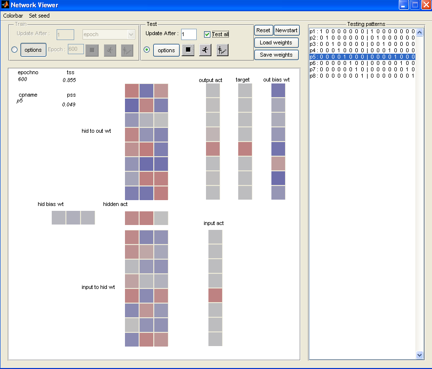
as output, through a distributed hidden representation. Over the course of this
tutorial, you will create a network that learns this mapping, with the finished
network illustrated in Figure B.3.
Creating a network involves four main steps, each of which is explained in a
section:
- Creating the network initialization script (Appendix B.1)
- Creating the example file (Appendix B.2)
- Creating the display template (Appendix B.3)
- Setting parameters in the initialization script (Appendix B.4)
There are also several additional features of the software that you may want to exploit in
running a simulation, and these are also covered in later sections:
- Logging and graphing network variables (Appendix B.5)
- Additional commands; using the initialization script as a Batch Process
Script (Appendix B.6)
- The PDPlog file (Appendix B.7)
B.1 Creating the Network Initialization Script
The first thing you need to do is create a network initialization script. This file
initializes your network (with or without the graphical user interface), creates pools
of units, connections, and a network that ties them together, associates a training
environment with the network, and launches the network. Details on creating the
screen layout of network variables (called the display template), the format of the
example files, and additional items that can be included in the initialization script
are described in later sections.
It may be best to create a new directory for your example. So, at the command
line interface type
mkdir 838example
Then change to this directory
cd 838example
Up-to-date copies of the pdptool software distribution have such a directory and files
that work, consistent with the tutorial information here. The template file in that
folder is arranged differently than the one described below.
B.1.1 Initializing and Quitting the Software With or Without the Gui
The first things we must do in the script is to declare that the net object we will be
creating in the script should be available as a global data structure so that we can
interact with it both within our script and in the command window, then initializing
the pdp software. In the example below we also make the software’s outputlog data
structure available, which allows us to give commands that interact with it as
well.
global net outputlog;
pdpinit(’gui’);
The example initializes the software to open the GUI. If you want to run your
network as a batch process, without opening the GUI, provide the string ’nogui’ to
the pdpinit command. In that case you will also want to terminate your file with the
command
pdpquit;
The pdpquit command will cause the program to clean things up and exit so that
you can start another pdptool process without interaction with existing data
structures. You should not end your initialization file with the pdpquit command if
you wish to use the GUI to control the program. In that situation, you can type
pdpquit on the command line to end the program, or click the quit botton near the
top left of the command window.
Note: The pdpquit command command does leave some variables around in your
workspace, but they are likely to get clobbered the next time you start the software.
Thus, it is best to save anything you want to save to a file before quitting the
software.
B.1.2 Defining the Network Pools
It is now time to define the pools you want in your network. The software
automatically creates one pool, called the bias pool, and numbered pool one. You will
specify each of your other pools, by using the pool command, specifying for each
pool a poolname, a size, and a pooltype. For the 8-3-8 encoder network we
have:
pool(’in’,8,’input’);
pool(’hid’,3,’hidden’);
pool(’out’,8,’output’);
As shown here, the first argument is a string that becomes the name of the pool.
The second argument is the number of units in the pool, and the third argument is
the pool type. Note that in general there can be more than one pool of each type.
Also note that a fourth type ’inout’ is allowed in some types of networks, but not in
bp networks.
In any case, the network now has four pools, which can be referred to either by
name (bias, in, etc.) or by number (pools(i), where i can range in our
case from 1 to 4, with 1 indexing the bias pool, 2 indexing the ’in’ pool,
etc.
B.1.3 Defining the Connections Between Pools
We now specify the connections between the pools. By default, the bias
pool is connected to all of the other pools, which means that all units have
modifiable biases. To specify the connections to the hidden pool from the input
pool and to the output pool from the hidden pool, we use the following
commands:
hid.connect(in);
out.connect(hid);
Note that the beginning of the command is the name of the pool that will receive
the connections, and the argument to the command is the name of the pool from
which the connections will project.
B.1.4 Creating the Network Object
Next we will actually create the network object. The command for this in our case
is:
net = bp_net([in hid out],seed,’wrange’,1);
The command takes two obligatory arguments, a list of pools and a seed. The list of
pools is enclosed in square brackets, and the pool names are used, without quotes.
The seed can be an integer, in which case you will get the same random sequence
each time the network is run. Alternatively it can be the value of a variable called
seed, set by a call to the uint32(randi(maxi)) function, if a random seed is
desired. maxi should be an integer such as 232 - 1 or 4294967295. So the
following command inserted before the bp_net command will get you a random
seed:
seed = uint32(randi(2^(32)-1));
It is also a good idea to specify the range of the initial weight values in the call to
the bp_net function, since the weights are initialized when the function is called. We
have used a wrange of 1 in the example. Other arguments can be specified in this
function, but they can also be specified later more explicitly, as discussed
below.
B.1.5 Associating an Environment and a Display template with the
Network
We are almost ready to launch our network, but we must also associate an
environment (set of input-output patterns) and a display template with it.
The following three commands will complete the launching of the network,
provided that the files containing the patterns and the template already
exist.
net.environment = file_environment(’838.pat’);
loadtemplate 838.tem
lauchnet;
Note that the file_environment command takes the file name argument in quotes
while the loadtemplate command takes the file name argument without
quotes.
Below we provide the full sequence of commands that you could put in your
initialization file to launch your network for interactive use (i.e., in ’gui’
mode). You can place these commands in a file with extension .m, such as
bp_838.m.
global net outputlog;
pdpinit(’gui’);
pool(’in’,8,’input’);
pool(’hid’,3,’hidden’);
pool(’out’,8,’output’);
hid.connect(in);
out.connect(hid);
seed = uint32(randi(2^(32)-1));
net = bp_net([in hid out],seed,’wrange’,1);
net.environment = file_environment(’838.pat’);
loadtemplate bp_838.tem;
launchnet;
Once your pattern and template files exist, you can then run the script by
typing the filename (without the extension) at the MATLAB command
prompt.
We now turn to specifying how to create the pattern and template files.
B.2 Format for Pattern Files
Version 3 of the PDPtool software offers a rich format for specifying complex training
environments, which can involve extended sequences of inputs and targets provided
at different times. Full documentation of these features is available on the
PDPTool Wiki. Right click here and select ’open in new tab’ to access this
information.
Here we indicate the simple format that can be used to specify pattern files for
use with the bp program when there is only one input and one output pool. In this
case, each line of the file contains an optional pattern name in [] followed by a list of
input activation values, then the | (pipe) character, then a list of target values for the
output units. In the case of the 8-3-8 encoder network, then, the first two lines of the
file look like this:
[p1] 1 0 0 0 0 0 0 | 1 0 0 0 0 0
[p2] 0 1 0 0 0 0 0 | 0 1 0 0 0 0
B.3 Creating the Display Template
A graphical template construction window is provided for creating the display
template to use with your network. This window will automatically open if you
execute your network initialization script and: (1) the ’gui’ option is specified in the
pdpinit command and (2) no loadtemplate command has been executed before the
launchnet command is reached. Thus, you can cause this window to open
by running the script we have specified thus far with the loadtemplate
command omitted or commented out. (Comments begin with the % character in
MATLAB).
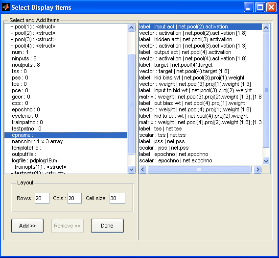
The window is broken into two panels: the left panel is a tree-like structure of
network objects that you can add to the display template and the right panel is your
current selection of such objects.
Start by clicking “+ net: struct” since the “+” indicates it can be expanded. This
shows many of the network parts. You can add network parts that you want
displayed on the template. For each item you want displayed, you can separately add
a “Label” and “Value” to the Selected Items panel. The Value will be a vector,
matrix, or scalar that displays the variable of interest. The Label will be placed in a
text box that can be placed near the value or values it labels to indicate which item
is which on the display.
What items do you want in your template? For any network, you may
want the activations of the pools displayed (except for the bias pool). This
allows you to see the pattern presented and the network’s response. For
many networks, if the pools are small enough (say less than 10 units each),
you may want to display the weights to see how the network has solved the
problem. Otherwise, you can ignore adding the weights, and you can always
use the MATLAB command window to view the weights if desired during
learning.
For our auto-encoder, we will want to display the pool activations, the target
vector, the weights and biases, and some summary statistics. Each of these items can
be accompanied by a label. We’ll walk you through adding the first item,
and then the rest are listed so you can add them yourself. Let’s start by
adding the activation of the input layer, which is named pools(2).activation.
Expand the pools(2) item on the left panel, and highlight the activation field.
The click the Add button. You must now select whether you want to add
a Label or Value. We will add both for each object. Thus, since Label is
already selected, type the desired label, which should be short (we use “input
act”). Click “Ok”. The label you added should appear in the right panel. All
we did was add a text object that says “input act,” now we want to add
the actual activation vector to the display. Thus, click Add again on the
pools(2).activation field, select Value, and set the Orientation to Vertical.
The orientation determines whether the vector is a row or column vector
on the template. This orientation can be important to making an intuitive
display, and you may want to change it for each activation vector. Finally,
set the vcslope parameter to be .5. Vcslope is used to map values (such
as activations or weights) to the color map, controlling the sensitivity of
the color around zero. We use .5 for activations and .1 for weights in this
network. Note that for vectors and arrays it is possible to specify that a display
object should be a part of a vector. This can come in handy when vectors get
long.
For the auto-encoder network, you may follow the orientations specified in the list
below. If you make a mistake when adding an item Value or Label, you can highlight
it in the right panel and press “Remove”.
Now it’s time to add the rest of the items in the network. For each item, follow all
the steps above. Thus, for each item, you need to add a Label with the specified text,
and then the Value with the specified orientation. We list all of these items below,
where the first one is the input activation that we just took care of. For each we give
a selected text string for the label and selected attributes associated with the display
of the variable.
pools(2).activation (Label = input act; Orientation = Vertical; vcslope = .5)
pools(3).activation (Label = hidden act; Orientation = Horiz; vcslope = .5)
pools(4).activation (Label = output act; Orientation = Vertical; vcslope = .5)
pools(4).target (Label = target; Orientation = Vertical; vcslope = .5)
pools(3).projections(1).using.weights (Label = hid bias wt; Orientation = Horiz; vcslope = .1)
pools(3).projections(2).using.weights (Label = input to hid wt; Transpose box checked; vcslope = .1)
pools(4).projections(1).using.weights (Label = out bias wt; Orientation = Vertical; vcslope = .1)
pools(4).projections(2).using.weights (Label = hid to out wt; Transpose box Un-checked; vcslope = .1)
tss (Label = tss)
pss (Label = pss)
epochno (Label = epochno)
cpname (Label = cpname)
Your screen should look similar to Figure B.1 when you are done adding the items
if you actually add all of them.
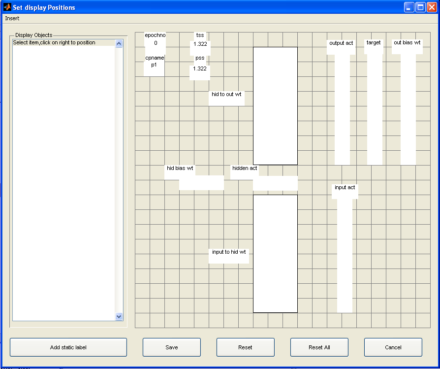
After adding the items you want to include in your template, click “Done”. The
“Set display Positions” screen should then pop-up, where you get to place the items
on the template. One intuitive way to visualize this encoder network is shown in
Figure B.2; the orientations specified in the list above are consistent with this
visualization.
To place an item on the template, select it on the left panel. Then, right click on
the grid to place the item about there, and you can then drag to the desired position.
If you want to return the item to the left panel, click “Reset” with the item
highlighted. If you selected the wrong orientation for the item, there’s an easy fix.
Simply save the template, click “Select display items...” on the main pdp
menu, and then remove and re-add the item with the proper orientation.
Pressing “Done” should then allow you to continue placing items as you were
before.
Once you have finished placing all of the selected items in the display, click Save
to save your template file. Your network will then load the template file
automatically, and you are ready to use it! However, you may just want to quit from
the network viewer, and make sure you have added or uncommented the
line
loadtemplate bp_838.tem
in the bp_828.m file just before the lauchnet command. The next section
describes additional commands you may want to place in your initialization
script.
B.4 Setting Parameters in the Initialization Script and Loading Saved
Weights
You will want to set training options that are reasonable for your network; while you
can do this through the train options button in the Gui while exploring things, it is
best to set the values of parameters in the initialization script so that you have a
record of them. We will indicate the command syntax of this with the lrate
parmeter:
net.train_options.lrate = .1;
You can also type commands such as these in the MATLAB Command Window
once you have started your network, and such commands are saved in the PDPlog
file, discussed below.
The list of available parameters for use in training may be viewed by simply
typing net.train_options in the command window, and a virtue of this that you
will see the settings as they have been set so far, either by default or by previous
commands. Another good way to see the relevant parameters is to open the ’options’
window within the ’train’ panel on the GUI. (You can view test options in the
analogous manners).
As an example, we might see from the train options that there is an option called
’errmeas’. The possible values of this option can be found by clicking on the little
dropdown menu next to this option in the GUI. The first listed option is the default,
and other options are shown. For the ’errmeas’ we see that the default is ’sse’ for
sum squared error, and there is an alternative ’cee’ for cross entropy error.
To specify that we want ’cee’ we could select it here, or we could type the
command
net.train_options.errmeas = ’cee’;
If we place this command in the script, we will then use it each time the script is
called.
A special case exists for one variable, the ’training mode’ variable. This variable is
a property of the environment, and it can be viewed by typing net.environment. It
can bet set as follows:
net.environment.trainmode = ’o’;
Where ’o’ is a character specifying one of the available options. The options in this
case are ’s’ for sequential (patterns are presented in the order encountered in the
environment), ’r’ for random (each time a new pattern is chosen a random selection is
made from the environment) and ’p’ for permuted (at the beginning of each epoch
the order of patterns is randomized; the patterns are then presented, once each per
epoch, in the random order specified). This is generally the preferred mode
when you are updating the weights after each pattern, which is specifyied by
setting the ’lgrain’ to ’pattern’ and the ’lgrainsize’ to 1. Below we show the
full set of non-default parameter settings used in the provided bp_838.m
file:
net.train_options.nepochs = 30;
net.train_options.lgrain = ’pattern’; %or ’epoch’
net.train_options.lgrainsize = ’1’;
net.train_options.errmeas = ’sse’; % or ’cee’;
net.train_options.lrate = 0.1;
net.environment.trainmode = ’p’; % ’s’ for sequential; or use
% ’r’ for random or ’p’ for permuted
Note that some parameters are present in the list of options or in the GUI, but
are not actually used in a given program. You can take a look at the chapter of the
handbook describing the particular model you are using to learn more about the
parameters that are used in a given program.
One other thing one often does in the initialization script is to load previously
saved weights. The command for this is simple; for example if we previously saved a
file named bp_838.wts, we would simply type:
loadweights(’bp_838.wts’);
B.5 Logging and Graphing Network Variables
There is a function built into the software that allows you to save the values of
various network variables to a log file, and other functions for displaying graphs of
selected variables as the network is running. For example, consider the following
commands. The first command creates a filename beginning with the name
’myname’, then a number not previously used (first time the process runs this
number will be 1), then the extension ’.mat’ – If you wish to save the file in text
format use the ’.out’ extension). The second command specifies the contents and
behavior of the log via a set of ’name’ - ’value’ pairs, where ’name’ is the name of a
variable and ’value’ is the value to assign to it. Finally, the last command specifies
parameters of the graph that will be created, if the ’plot’ variable has been set to
’on’.
trlogfname = getfilename(’838train’,’.mat’); % use ’.out’ for text file
setoutputlog (’file’,trlogfname,’process’,’train’,’frequency’,’epoch’,...
’status’, ’on’, ’writemode’,’binary’,’objects’,{’epochno’,’tss’},...
’onreset’, ’clear’, ’plot’, ’on’,’plotlayout’, [1 1]);
setplotparams (’file’, trlogfname, ’plotnum’, 1,’yvariables’, {’tss’});
In summary, we have created a unique file name for the log we will create,
in case a log from a previous run already exists. We then set up the log
itself, with a series of attribute-value pair arguments, and finally we set
up the parameters of the plot we will display when running the software
interactively.
We now consider the arguments to the setoutputlog and setplotparams
commands in more detail.
Here is a list of the attribute-value pairs for the setoutputlog command. The
first value listed is the default when applicable.
Attribute -- Value Pairs for Setoutputlog
Attribute Value
’file’ string name of file
’process’ {’train’,’test’}, ’train’,’test’
’frequency’ ’pattern’, ’epoch’ or ’patsbyepoch’
’status’ ’off’,’on’
’writemode’ ’binary’, ’text’
’objects’ list of net var names in single quotes inside {}
for vector/matrix values, ranges may be specified
’onreset’ ’clear’, ’startnew’ see below
’plot’ ’off’,’on’ - always off in nogui mode
’plotlayout’ [row col] specification indicating the
layout of subwindows in the plot window
Most of the above should not need further explanation. the ’patsbyepoch’ option for
frequency, however, is a special case. It allows the logging of activations for each
pattern once per epoch, and this is used in one of the graphs provided with the
bp_xor exercise. The ’onreset’ attribute determines what happens when the reset
or newstart commands are executed. With the default, ’clear’ value, the log and
associated graphs are cleared and reused. With the alternative ’startnew’ value, the
log is closed, any graphs remain open, a new log is created with ’_n’ added to the file
name (where n increments with each reset/newstart) and new graphs are
initialized.
As with training options, you can inspect the properties of your output log or
logs. They are numbered sequentially in a structure called outputlog. To inspect the
values associated with the above created output log, for example, you can
type:
outputlog(1)
To turn off logging in an output log, you could type:
outputlog(1).status = ’off’;
Alternatively a log can be turned off by calling the setoutputlog command with the
file and status attribute value-pairs as follows:
setoutputlog(’file’,trlogfname,’status’,’off’);
The commands to the setoutputlog command also specify that we want to plot
some of the objects in our log within a plot window (MATLAB figure environment)
associated with the log. To specify what to plot within each subwindow, one uses the
setplotparams command. The attribute-value pairs for this commend are shown
below.
Attribute -- Value Pairs for Setplotparams
Attribute Value
’file’ string name of file
’plotnum’ panel number within [r c] grid specified
in log; increases across row first
’yvariables’ list of var names in single quotes inside {}
ranges may be specified as above
’title’ text string
’ylim’ [ymin ymax]
’plot3d’ set to 1 for 3d plot
’az’ azimuth of view on 3d plot
’el’ elevation of view on 3d plot
The first two arguments listed essentially address the log and sub-plot within the
figure associated with the log, and the remaining arguments specify attributes of this
particular subplot. In the example shown previously, we have only one subplot, so its
’plotnum’ is 1. The x axis of the plot will be determined by the ’frequency’ field of
the log, and the range of the x axis updates automatically as the count associated
with the variable (e.g., the epochno) increases. The ’yvariables’, ’title’, and ’ylim’
fields should be self-explanatory. The last three arguments allow for 3-d offset of
lines being plotted, which is helpful for visualization when there are many
lines on a plot. These options are specified in the iac_jets.m file for the
corresponding exercise, and that file can be consulted for an example of their
use.
Selected weights in your network can be logged, just like other variables, but more
common is to save weights using a special command for this action, because it saves
the entire weight structure in a format suitable for reloading into you network. An
example follows.
wfname = filename(’838weights’,’.wt’)
saveweights(’file’,wfname,’mode’,’b’); %mode can be ’a’ CHECK!
This will create a unique filename for the weights file with a sequantially increasing
number, so that previous files will not be overwritten. Alternatively you can directly
specify a string name in quotes in place of the wfname variable name in the
saveweights command.
B.6 Additional Commands; Using the Initialization Script as a Batch Process
Script
In addition to commands already discussed, one may put a list of additional
commands in the initialization script, including standard MATLAB code. Simply by
setting ’nogui’ in the pdpinit command, the script becomes a batch process control
script that can be run without any input from the user. (It is even possible to open a
separate MATLAB process and continue using Matlab tools while your process is
running). Below we give an example of a set of commands one might append to the
initialization script above if one wished to save results of testing the 838 network at
different time points during learning, and also save the weights at the same time
points.
%set up test logging for batch process, saving epochno, pattern name, pss,
%and hidden unit activations (pools(3) is the hidden unit pool)
tstlogfname = getfilename(’838ttest’,’.mat’);
setoutputlog(’file’,tstlogfname,’process’,’test’,’status’,’on’,’writemode’,...
’binary’,’plot’,’off’,’objects’,{’epochno’,’cpname’,’pss’,’pools(3).activation’});
% now we begin processing, first testing the network before training, then
% testing and saving weights after increasing numbers of processing steps
runprocess (’granularity’,’pattern’,’count’,1,’alltest’,1,’range’,[]);
% run the test process (the default process) on all items
for i = 1:5 %loop 5 times, training, testing, then saving the weights at increasing intervals
runprocess(’process’,’train’,’granularity’,’epoch’,’count’,1,’range’,[]);
runprocess (’granularity’,’pattern’,’count’,1,’alltest’,1,’range’,[]);
wfile = getfilename(’838weights’,’.wt’); %gets a new file name with a
%unique number in its name
saveweights(’file’,wfile,’mode’,’b’); %saves weights to this file.
net.train_options.nepochs = 2*net.train_options.nepochs; %double number
%of epochs to train for next iteration
end %end of for loop
pdpquit; %quit program, close logs, and clean up gracefully
B.7 The PDPlog file
A final thing to note is that every time a pdp program runs, a logfile is created in
the directory from which the process is run. These log files have unique
sequential numerical names. The content of these files contains a record of
commands executed at the command line (including the calling command, which
indicates the script file name that was called) and some of the commands
executed in the script and through the gui. Thus, this file can be used to
provide a record of the steps one has taken during an interactive run, and even
as a base for creating a subsequent script for a batch run. However, there
are some limitations. Option-setting actions you take when setting values
of options through the train or test options are not currently logged, and
only some of the commands in your initialization/batch script are currently
being logged. Setting options via the command window ensures that they are
logged. Note that any command typed is logged, including typos, so you
should be aware of that if you plan to use this log as the basis of a batch
file.