2. As an example, consider the flow in a
channel that is 1000 m long in which two boundaries are specified as inflow and outflow and the other two
are specified as solid walls, as shown in Figure 2.
|
.5 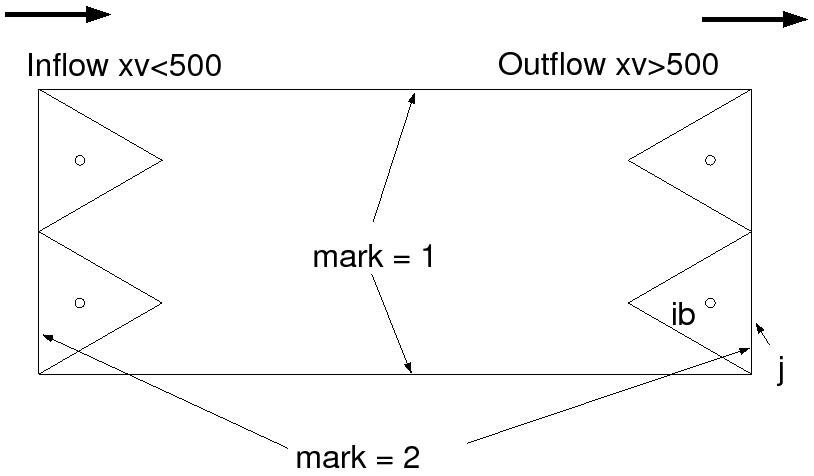
|
boundaries.c file as follows
  for(jptr=grid->edgedist[2];jptr<grid->edgedist[3];jptr++) {
    j = grid->edgep[jptr];

    ib = grid->grad[2*j];

    if(grid->xv[ib]>500) {
      for(k=grid->etop[j];k<grid->Nke[j];k++)
         ub[j][k] = -phys->h[ib]*sqrt(prop->grav/(grid->dv[ib]));
    } else {
      for(k=grid->etop[j];k<grid->Nke[j];k++)
         ub[j][k]=phys->boundary_u[jptr-grid->edgedist[2]][k]*grid->n1[j]+
                  phys->boundary_v[jptr-grid->edgedist[2]][k]*grid->n2[j];
    }
 }
  for(jptr=grid->edgedist[2];jptr<grid->edgedist[3];jptr++)
    j = grid->edgep[jptr];

    ib = grid->grad[2*j];

    if(grid->xv[ib]>500) {
      for(k=grid->etop[j];k<grid->Nke[j];k++) {
        phys->boundary_u[jptr-grid->edgedist[2]][k]=phys->uc[ib][k];
        phys->boundary_v[jptr-grid->edgedist[2]][k]=phys->vc[ib][k];
        phys->boundary_w[jptr-grid->edgedist[2]][k]=
            0.5*(phys->w[ib][k]+phys->w[ib][k+1]);
      }
    } else {
      for(k=grid->etop[j];k<grid->Nke[j];k++) {
        phys->boundary_u[jptr-grid->edgedist[2]][k]=
            prop->amp*cos(prop->omega*prop->rtime);
        phys->boundary_v[jptr-grid->edgedist[2]][k]=0;
        phys->boundary_w[jptr-grid->edgedist[2]][k]=0;
        }
    }
 }
jptr loop loops over the edges which have boundary markers specified as 2.
The j index is an index to an edge along the open boundary, and
the ib index is an index to the cell adjacent to that boundary edge. Since the Voronoi points
are specified at the ib indices, then we need to specify the boundary condition based on
the location of the Voronoi points of the adjacent cell. In this case the open boundary exists at x=1000, but since
we know that this boundary exists for boundary edges for if(grid->xv[ib]>500) to specify these boundary edges. The first part of the if statement
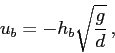
sets the flux at the open boundary over all the vertical levels with
      for(k=grid->etop[j];k<grid->Nke[j];k++)
        ub[j][k] = -phys->h[ib]*sqrt(prop->grav/(grid->dv[ib]));
which is identical to
Nke[j] variable, which is the number of vertical levels at face j,
and etop[j], which is the index of the top level at the boundary. The variable
etop[j] is usually 0 unless filling and emptying occur at the boundary
edges.
In addition to setting
the boundary flux in the OpenBoundaryFluxes function, the user must also set the Cartesian components
of velocity in the BoundaryVelocities function. These are used to compute the advection of momentum.
They can also be used to specify boundary velocities for no-slip type 4 boundary conditions.
At the open outflow boundary, the boundary velocity components are set to the upwind value of the velocity
component. For the u-component of velocity, for example, the boundary value is specified
with
phys->boundary_u[jptr-grid->edgedist[2]][k]=phys->uc[ib][k];Here,
uc is the u-component of velocity at the Voronoi point with index ib.
At the inlet, only the Cartesian velocity components need to be specified. In this example, the u-component of velocity at the inlet is set with the code
phys->boundary_u[jptr-grid->edgedist[2]][k]=
               prop->amp*cos(prop->omega*prop->rtime);
and the other components are set to 0. This function uses the variables amp and omega
which are set in suntans.dat, and rtime is the physical time in the simulation.
The Cartesian velocities which are specified at the inlet boundary are then used to compute
the flux in the OpenBoundaryFluxes function with
ub[j][k]=phys->boundary_u[jptr-grid->edgedist[2]][k]*grid->n1[j]+
         phys->boundary_v[jptr-grid->edgedist[2]][k]*grid->n2[j];
This is just the dot product of the velocity field specified at the boundary with the
normal vector at the boundary edge, which points into the domain by definition.
Examples of how to employ velocity boundary conditions are described in Sections 6.5
and 6.7. Section 6.5 also demonstrates
how to specify salinity and temperature at the boundaries.