The grid for this example was generated with GAMBIT and is shown in Figure 3
(for tips on using GAMBIT for SUNTANS please see
http://suntans.stanford.edu/documentation/suntans_tutorial.pdf).
Grids like this can be generated by obtaining a coastline from the NOAA coastline extractor
http://rimmer.ngdc.noaa.gov/coast/
and reading it into a grid generation program after converting the coordinates to a Cartesian grid.
Most grids in SUNTANS are obtained with a UTM projection, but for larger grids that cross over multiple
UTM zones, the Mercator projection is also suitable.
Upon running SUNTANS (with -g -vv), Voronoi distance statistics will be output as follows:
Voronoi statistics:
        Minimum distance: 1.97e+02
        Maximum distance: 4.43e+03
        Mean distance: 2.85e+03
        Standard deviation: 4.14e+02
Note that while the minimum distance in this example is acceptable, the Voronoi distances do
not indicate whether there are degenerate cells in the domain (i.e. obtuse triangles). In order
to correct for any degenerate triangles, the parameter CorrectVoronoi is set to -1,
and the parameter VoronoiRatio is set to 85 degrees (these parameters are in suntans.dat).
This corrects any triangles
with angles greater than 85 degrees by placing the Voronoi points at the triangle centroids.
After correction, the statistics are displayed as
Corrected 11 of 1534 cells with angles > 85.0 degrees (0.72%).
Voronoi statistics after correction:
        Minimum distance: 9.49e+02
        Maximum distance: 4.34e+03
        Mean distance: 2.85e+03
        Standard deviation: 3.95e+02
This highlights the fact that 11 cells in the grid were obtuse and were corrected. Also note that
as a result of the correction the minimum distance between Voronoi points increased from 197 m to
949 m. This substantially raises the minimum allowable time step for stability of the nonlinear
advection terms.
|
0.75 
|
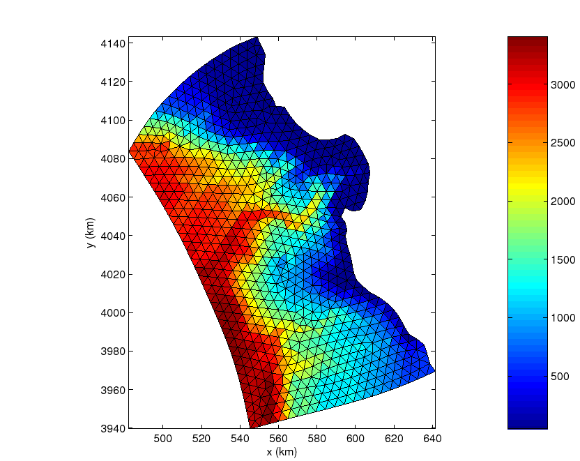
For the bathymetry, 250 m resolution bathymetry is available in the file
rundata/mbay_bathy.dat which was obtained from the MBARI multibeam survey
http://www.mbari.org/data/mapping/monterey/default.htm
This file is specified by the depth variable in suntans.dat.
The interpolated bathymetry is depicted in Figure 4.
Upon running SUNTANS, bathymetry from this file is interpolated onto the (possibly corrected) Voronoi points.
Because this procedure can take quite some time, it is a good idea to only run it when necessary and use
the pre-interpolated bathymetry for subsequent runs. Each time SUNTANS interpolates bathymetry, it outputs
the interpolated bathymetry into the file mbay_bathy.dat-voro (it appends ``-voro'' to the specified
bathymetry file). This file is created when the variable IntDepth is set to 1 in suntans.dat.
Otherwise, if this variable is set to 2, data is not interpolated but instead is read in from the -voro file.
Note that any time changes are made to the Voronoi points, the bathymetry should be re-interpolated.