This example is run by typing make test in the suntans/main/examples/tides directory.
This will compile the boundary conditions specified in boundaries.c
and link them with the main sun executable, and then run the test. Data is copied from
the rundata directory to the data directory, which becomes the working directory. Typing
make test again only copies rundata/suntans.dat to data/suntans.dat and runs
the example again. Therefore, if any changes that are made to the grid or any associated parameters,
the directory should be flushed with make clobber. This ensures that typing make test will
recompute the grid.
Upon running the tidal example, the simulation will
complain that the tidal input files (as specified by TideInput in suntans.dat)
are not present, with the error message
Error opening data/tidecomponents.dat.0!
Writing x-y boundary locations to data/tidexy.dat.0 instead.
Error opening data/tidecomponents.dat.1!
Writing x-y boundary locations to data/tidexy.dat.1 instead.
In order to create these files (for details see Section 6.2.3), run the matlab script
tides.m. This script will read in the locations of the boundary points
in the tidexy.dat.* files and output the required tidecomponents.dat.* files. In order
to run this script, the paths to the required m-files must be specified in the file
setup_tides.m. These are given by
addpath ../../../mfiles
addpath ../../../mfiles/suntides
addpath /home/fringer/research/SUNTANS/tides/m_map
The first two paths should not need to be changed since these represent the default locations of the suntans mfiles and suntides directories. However, the user must set the location of the path to the m_map directory, which contains routines to convert from lon/lat coordinates to Cartesian coordinates using the UTM projection. This package can be downloaded from
http://www.eos.ubc.ca/~rich/map.html
Note that the data directory in the suntides directory must also be unpacked in order to run
the suntides.m script. This can be done by typing make in the suntans/mfiles/suntides directory.
Running the tides.m script will generate the tidecomponents.dat files
and will display the following message:
File ./data/tidexy.dat.0, found 40 boundary points.
File ./data/tidexy.dat.1, found 32 boundary points.
This indicates that the locations of the boundary edges were found in the files
tidexy.dat.* and these
were output into the tidecomponents.dat.* files in the data directory.
Once these files have been created, the example can be run with make test, which will proceed as
follows:
Running suntans...
Processor 0,  Total memory: 1.77 Mb, 3865 cells
All processors: 3.58 Mb, 7719 cells (474 bytes/cell)
Outputting data at step 1 of 13440
5% Complete. 5.11e-02 s/step; 652.11 s remaining.
Outputting data at step 1344 of 13440
10% Complete. 4.85e-02 s/step; 587.19 s remaining.
15% Complete. 4.68e-02 s/step; 534.33 s remaining.
Outputting data at step 2688 of 13440
.
.
.
This indicates that the simulation (which by default runs on two processors) takes 0.05 seconds per time step to run, which is 1800 times faster than real time (since the time step, as specified by the
dt variable in suntans.dat is 90 s). Data is output every 1344 time steps as
indicated by the ntout variable in suntans.dat. The simulation will run for a total
of nsteps=13440 time steps or a total simulation time of nsteps*dt=14 days. Note
that the values of the horizontal (nu_H) and vertical (nu) eddy-viscosities (called ``laminar'' because they
are constant) are large in order to prevent the buildup of grid-scale energy over the course of
the simulation on a relatively coarse grid.
Output of the results can be viewed with the compare_to_otis.m matlab script
(which requires the correct path locations in setup_tides.m).
This script compares the results of SUNTANS to the OTIS results at the location specified in the file
data/dataxy.dat (in UTM coordinates). For details on how to specify these points
and analyze data from these points, see the header in the file suntans/main/profiles.c and the
associated mfile suntans/mfiles/profplot.m. The associated
lines in the present example in suntans.dat are given by
########################################################################
#
# For output of data
#
########################################################################
ProfileVariables        hu    # Only output free surface and currents
DataLocations   dataxy.dat    # dataxy.dat contains column x-y data
ProfileDataFile profdata.dat  # Information about profiles is in profdata.dat
ntoutProfs              1     # Output profile data every 1 time step
NkmaxProfs              1     # Only output the top 1 z-level
numInterpPoints         1     # Output data at the nearest neighbor.
These indicate that free surface and velocity data at the locations specified in the file
dataxy.dat
will be output every time step (ntoutProfs). Because NkmaxProfs is set to 1, only the
top cell is output. Otherwise, if NkmaxProfs is zero, all layers are output (this example has
Nkmax=10 layers). The numInterpPoints variable indicates how many of the points nearest to
the desired point are output. SUNTANS does not interpolate output data; this is left up to the user.
In the present example it suffices to output nearest-neighbor data. The output data can be compared to
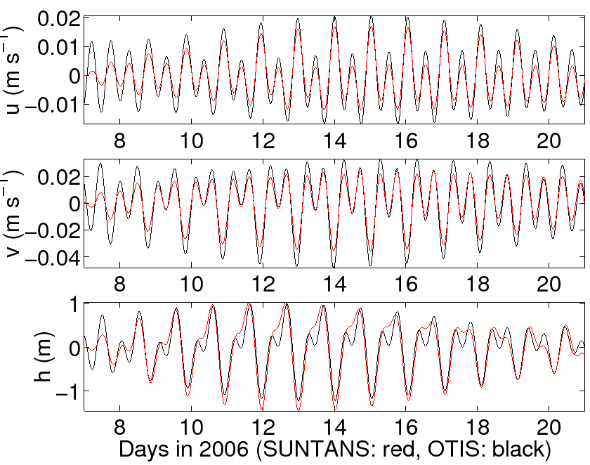
the predictions of OTIS with the script compare_to_otis.m. Over the 14-day
period, the results are given in Figure 5. It should be noted that because
the OTIS data used for this example is quite coarse (1 degree) and because the interpolation used to
obtain the constituents near the coastline can lead to inaccurate predictions of the tidal boundary conditions
in the shallow areas of the domain, this comparison should not be regarded as a measure of the accuracy
of SUNTANS tidal simulations. The user is encouraged to obtain higher-resolution tidal data for more accurate
simulations. For more detail please visit Brian Dushaw's web page2.
To highlight the differences associated with the coarse tidal data, Figure 6 compares
the results of SUNTANS when employing three different interpolation techniques to obtain the tidal data
at the SUNTANS boundaries. The particular interpolation method can be changed in the function suntans/mfiles/suntides/get_tides.m,
and the results are strikingly different because the interpolation method has a significant effect on
forcing values near the coastline, since it is assumed that land values from OTIS are identically zero.
|
0.75 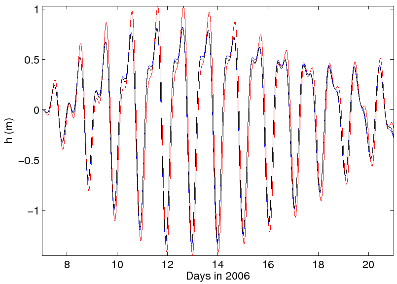
|