Negative stepsizes also make multi-block ADMM converge
This blog post investigates the idea from a recent advance (Shugart and Altschuler 2025) from minimax optimization: by periodically using negative stepsize, vanilla gradient descent ascent can be made to converge on the conventional counterexamples. (Shugart and Altschuler 2025) provides an explanation that negative stepsizes can provide a “slingshot” effect and introduces a second-order effect. This interesting phenomenon makes the author wonder whether the idea can be generalized beyond minimax optimization, especially whether negative stepsize allows bypassing certain counterexamples for other algorithms. In the ADMM literature, there is a well-known counterexample (Chen et al. 2016) that demonstrates divergence of multi-block ADMM on simple quadratic functions. We show that periodic negative stepsize on the ADMM dual update allows multi-block ADMM to converge on the counterexample instances.
Introduction and background
In a recent work (Shugart and Altschuler 2025) on minimax optimization, it is shown that gradient descent ascent can escape the bilinear counterexamples by employing a special stepsize rule. There are several components in the stepsize rule from (Shugart and Altschuler 2025), and probably the most notable one is the negative stepsize. For simplicity, we explain the idea in the quadratic minimization context.
Consider a toy quadratic minimization problem \[ \min_{x \in \mathbb{R}^n} \quad f(x) := \tfrac{1}{2} \langle x - x^{\star}, \Lambda (x - x^{\star}) \rangle, \] where \(\Lambda = \begin{pmatrix} \lambda_1 & & \\ & \ddots & \\ & & \lambda_n \end{pmatrix}\) is a positive definite diagonal matrix with \(L := \lambda_1 \geq \lambda_2 \geq \cdots \geq \lambda_n =: \mu > 0\).
Consider the gradient descent iteration with stepsize \(\alpha \geq 0\): \[ x^+ = x - \alpha \nabla f(x). \tag{1}\label{eq-gd} \] We obtain, after subtracting both sides by \(x^{\star}\) and using \(\nabla f(x) = \Lambda(x - x^{\star})\), that \[ x^+ - x^{\star} = x - x^{\star} - \alpha \nabla f(x) = x - x^{\star} - \alpha \Lambda (x - x^{\star}) = (I - \alpha \Lambda)(x - x^{\star}), \] where \(\alpha\) is the stepsize. Since \(\lambda_{\max}(\Lambda) = L\) and \(\lambda_{\min}(\Lambda) = \mu\), we have \[ \| I - \alpha \Lambda \| = \left\| \begin{pmatrix} 1 - \alpha L & & \\ & \ddots & \\ & & 1 - \alpha \mu \end{pmatrix} \right\| = \max\{|1 - \alpha L|,\, |1 - \alpha \mu|\}. \] If \(\|I - \alpha \Lambda\| < 1\), then \(\|x^+ - x^{\star}\| \leq \|I - \alpha \Lambda\| \|x - x^{\star}\|\) and gradient descent converges. Clearly, \(\|I - \alpha \Lambda\| < 1\) if and only if \(\alpha \in \left(0, \tfrac{2}{L}\right)\).
Negative stepsize. The idea of using a negative stepsize is simply reverting the direction of update in \((\ref{eq-gd})\): \[ x^+ = x + \alpha \nabla f(x). \] Repeating the same argument as above, we have \(x^+ - x^{\star} = (I + \alpha \Lambda)(x - x^{\star})\). However, we always have \(\lambda_{\min}(I + \alpha \Lambda) > 1\) and a negative stepsize inevitably leads to divergence.
What if we alternate between a positive and a negative stepsize? Say we take \(\alpha \geq 0\) and \[ x^{++} = x^+ + \alpha \nabla f(x^+), \quad x^+ = x - \alpha \nabla f(x). \] If we focus on per-iteration progress, then every time a negative stepsize is taken, divergence happens. However, if we analyze two steps at the same time, things become slightly different. We can write
\[ \begin{aligned} x^{++} - x^{\star} &= (I + \alpha \Lambda)(x^+ - x^{\star}) \\ &= (I + \alpha \Lambda)(I - \alpha \Lambda)(x - x^{\star}) \\ &= (I - \alpha^2 \Lambda^2)(x - x^{\star}) \end{aligned} \]
and \(\|I - \alpha^2 \Lambda^2\| \leq 1\) if \(\alpha \in \left(0, \tfrac{\sqrt{2}}{L}\right)\). Therefore, gradient descent still converges if it alternates between a positive and a negative stepsize. But negative stepsize clearly does not give any benefits in the quadratic case: since \(|1 - x^2| \geq |1 - x|\) when \(x \in (0, \sqrt{2})\), we always have \(|1 - \alpha^2 \lambda_k^2| \geq |1 - \alpha \lambda_k|\).
Although the quadratic example does not show benefits of using a negative stepsize, two insights from its analysis will be useful.
It is useful to analyze the progress of an algorithm for more than one iteration.
A single negative causes divergence, but when we analyze two iterations, convergence is restored.
Some cancellation happens when alternating between positive and negative stepsizes. In particular, \[ (I + \alpha \Lambda)(I - \alpha \Lambda) = I - \alpha \Lambda + \alpha \Lambda - \alpha^2 \Lambda^2 = I - \alpha^2 \Lambda^2. \]
Now, we will move to the formal question in this post. Since negative stepsize is known to be useful in minimax optimization and allows gradient descent-ascent to escape the counterexample,
Can we find another instance to demonstrate the usefulness of negative stepsize?
The answer, as the title suggests, is the alternating direction method of multipliers (ADMM).
Multi-block ADMM
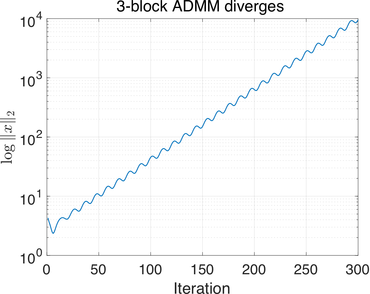
Consider the constrained optimization problem \[ \min_{\{x_i\}} \quad \sum_{i=1}^m f_i(x_i) \qquad \text{subject to} \quad \sum_{i=1}^m A_i x_i = b \quad (\lambda). \] One way of solving the problem is through alternating direction methods of multipliers (ADMM). Standard two-block (\(m = 2\)) version of ADMM is effective in both theory and in practice: \[ \begin{aligned} x_1^{k+1} &= \arg\min_{x_1} \left\{ f_1(x_1) + f_2(x_2^k) + \langle \lambda^k, A_1 x_1 + A_2 x_2^k - b \rangle + \tfrac{\rho}{2}\|A_1 x_1 + A_2 x_2^k - b\|^2 \right\} \\ x_2^{k+1} &= \arg\min_{x_2} \left\{ f_1(x_1^{k+1}) + f_2(x_2) + \langle \lambda^k, A_1 x_1^{k+1} + A_2 x_2 - b \rangle + \tfrac{\rho}{2}\|A_1 x_1^{k+1} + A_2 x_2 - b\|^2 \right\} \\ \lambda^{k+1} &= \lambda^k + \rho (A_1 x_1^{k+1} + A_2 x_2^{k+1} - b). \end{aligned} \] However, when the block number \(m \geq 3\), it is known that the direct extension of two-block ADMM to multi-block even cannot converge for a simple linear feasibility problem (Chen et al. 2016): \[ \begin{aligned} \min_{x_1, x_2, x_3} \quad & 0 \\ \text{subject to} \quad & \begin{pmatrix} 1 \\ 1 \\ 1 \end{pmatrix} x_1 + \begin{pmatrix} 1 \\ 1 \\ 2 \end{pmatrix} x_2 + \begin{pmatrix} 1 \\ 2 \\ 2 \end{pmatrix} x_3 = 0. \end{aligned} \tag{2}\label{eq-counterexample} \]
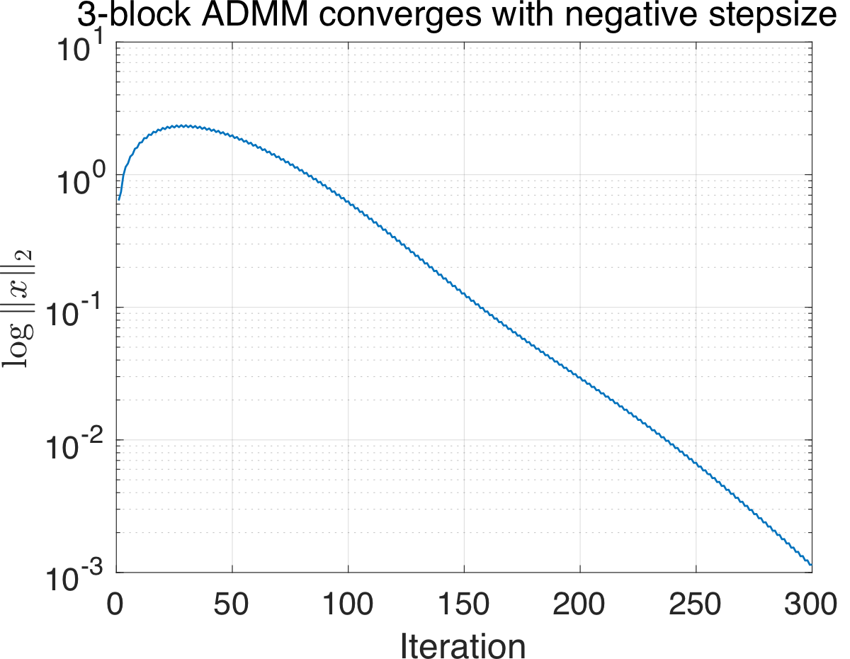
As Figure 1 (left) shows, three-block ADMM diverges on this simple instance. What if we try negative stepsize? The dual ascent step \(\lambda^{k+1} = \lambda^k + \rho \left(\sum_{i=1}^m A_i x_i^{k+1} - b\right)\) in ADMM looks like a good candidate for trying negative stepsize. So let’s replace it by \[ \lambda^{k+1} = \lambda^k + \rho \, {\color{red}(-1)^k} \left( \sum_{i=1}^m A_i x_i^{k+1} - b \right), \tag{3}\label{eq-admm-negstep} \] where we simply alternate between dual ascent and descent. Although it is a naive attempt, as Figure 1 (right) suggests, three-block ADMM with negative stepsize does converge.
The results so far are somewhat interesting but are fully empirical. The good news is that, the convergence behavior is not a coincidence. In fact, we can prove the following more general result:
Theorem 1 ADMM with (alternating) negative dual stepsize \((\ref{eq-admm-negstep})\) converges on linear feasibility problems: \[ \min_x \quad 0 \qquad \text{subject to} \quad Ax = b, \] where \(A \in \mathbb{R}^{n \times n}\) is full-rank.
We note that several well-known attempts that address divergence of ADMM (such as random permutation (Sun et al. 2020)) also start by considering this simple toy problem. For linear feasibility problem, the convergence analysis of ADMM can be reduced to analyzing the spectrum of some iteration matrix. And our analysis also proceeds in this vein. We leave the technical details to Section 2 in case it is of interest to some of the readers. But the main take-aways are summarized as follows:
- Negative stepsize does find its application beyond minimax optimization.
- For this particular ADMM case, alternating between positive/negative stepsizes cancels diverging components of the spectrum of two consecutive iteration matrices.
- Unfortunately, the average-case performance of multi-block ADMM seems not improved with negative stepsize alone.
Analyzing ADMM with negative stepsize
This section is devoted to the proof of Theorem 1 and we consider the following feasibility problem \[ \min_x \quad 0 \qquad \text{subject to} \quad Ax = b. \] The proof is mostly computation. We start by explicitly writing the ADMM iteration as a simple fixed-point iteration using the framework in (Sun et al. 2020).
\[ \begin{aligned} x_i^{k+1} = \arg\min_{x_i} \Bigl\{\ &\Bigl\langle \lambda^k,\ \sum_{j < i} A_j x_j^{k+1} + \sum_{j > i} A_j x_j^k + A_i x_i - b \Bigr\rangle \\ &+ \frac{1}{2} \Bigl\| \sum_{j < i} A_j x_j^{k+1} + \sum_{j > i} A_j x_j^k + A_i x_i - b \Bigr\|^2\ \Bigr\} \end{aligned} \tag{4} \]
\[ \lambda^{k+1} = \lambda^k + {\color{red}(-1)^k} \left( \sum_{i=1}^m A_i x_i^{k+1} - b \right) \]
Since the objective is constant \(0\), without loss of generality, we can assume \(\rho = 1\). (Otherwise we can scale the initial multiplier \(\lambda^1 \leftarrow \lambda^1 / \rho\).) The optimality condition of the subproblem gives
\[ \begin{aligned} & A_i^\top \lambda^k + A_i^\top \left( \sum_{j < i} A_j x_j^{k+1} + \sum_{j > i} A_j x_j^k + A_i {\color{red}x_i^{k+1}} - b \right) = 0 \\ \Rightarrow\quad & A_i^\top A_i {\color{red}x_i^{k+1}} = A_i^\top b - A_i^\top \lambda^k - A_i^\top \left( \sum_{j < i} A_j x_j^{k+1} + \sum_{j > i} A_j x_j^k \right). \end{aligned} \]
To understand the pattern of updates, let’s see what happens for \(m = 3\) with \(A = \begin{pmatrix} | & | & | \\ A_1 & A_2 & A_3 \\ | & | & | \end{pmatrix}\). Then
\[ \begin{aligned} A_1^\top A_1 x_1^{k+1} &= A_1^\top b - A_1^\top \lambda^k - A_1^\top (A_2 x_2^k + A_3 x_3^k) \\ A_2^\top A_2 x_2^{k+1} &= A_2^\top b - A_2^\top \lambda^k - A_2^\top (A_1 x_1^{k+1} + A_3 x_3^k) \\ A_3^\top A_3 x_3^{k+1} &= A_3^\top b - A_3^\top \lambda^k - A_3^\top (A_1 x_1^{k+1} + A_2 x_2^{k+1}) \\ \lambda^{k+1} &= \lambda^k + (-1)^k (A_1 x_1^{k+1} + A_2 x_2^{k+1} + A_3 x_3^{k+1} - b), \end{aligned} \]
re-arranging the terms to move terms with index \(k+1\) to the LHS,
\[ \begin{aligned} A_1^\top A_1 x_1^{k+1} &= A_1^\top b - A_1^\top \lambda^k - A_1^\top A_2 x_2^k - A_1^\top A_3 x_3^k \\ A_2^\top A_1 x_1^{k+1} + A_2^\top A_2 x_2^{k+1} &= A_2^\top b - A_2^\top \lambda^k - A_2^\top A_3 x_3^k \\ A_3^\top A_1 x_1^{k+1} + A_3^\top A_2 x_2^{k+1} + A_3^\top A_3 x_3^{k+1} &= A_3^\top b - A_3^\top \lambda^k \\ \lambda^{k+1} - (-1)^k (A_1 x_1^{k+1} + A_2 x_2^{k+1} + A_3 x_3^{k+1}) &= \lambda^k - (-1)^k b. \end{aligned} \]
Hence in matrix form, we have \[ \begin{pmatrix} A_1^\top A_1 & 0 & 0 & 0 \\ A_2^\top A_1 & A_2^\top A_2 & 0 & 0 \\ A_3^\top A_1 & A_3^\top A_2 & A_3^\top A_3 & 0 \\ A_1 & A_2 & A_3 & I \end{pmatrix} \begin{pmatrix} x_1^{k+1} \\ x_2^{k+1} \\ x_3^{k+1} \\ (-1)^{k+1} \lambda^{k+1} \end{pmatrix} = \begin{pmatrix} A_1^\top b \\ A_2^\top b \\ A_3^\top b \\ (-1)^{k+1} b \end{pmatrix} + \begin{pmatrix} 0 & -A_1^\top A_2 & -A_1^\top A_3 & -A_1^\top \\ 0 & 0 & -A_2^\top A_3 & -A_2^\top \\ 0 & 0 & 0 & -A_3^\top \\ 0 & 0 & 0 & I \end{pmatrix} \begin{pmatrix} x_1^k \\ x_2^k \\ x_3^k \\ \lambda^k \end{pmatrix}. \]
For brevity, we define \(L\) to be the block lower-triangular part of \(A^\top A\) and let \(\delta := (A^\top b,\, -b)\), \(\delta^- := (A^\top b,\, b)\). In the above example, \[ L = \begin{pmatrix} A_1^\top A_1 & 0 & 0 \\ A_2^\top A_1 & A_2^\top A_2 & 0 \\ A_3^\top A_1 & A_3^\top A_2 & A_3^\top A_3 \end{pmatrix}, \quad \delta = \begin{pmatrix} A_1^\top b \\ A_2^\top b \\ A_3^\top b \\ -b \end{pmatrix}, \quad \delta^- = \begin{pmatrix} A_1^\top b \\ A_2^\top b \\ A_3^\top b \\ b \end{pmatrix}. \]
Then the ADMM iterates can be written as linear fixed-point iterations.
Lemma 1 ((Sun et al. 2020), Section 3.1). Define the state variable \(z := (x_1, \ldots, x_m, -\lambda)\). Then
- If \(k\) is even, then \(z^{k+1} = M z^k + L^{-1} \delta\)
- If \(k\) is odd, then \(z^{k+1} = M^- z^k + L^{-1} \delta^-\),
where the iteration matrices are \[ M := \begin{pmatrix} L & 0 \\ A & I \end{pmatrix}^{-1} \begin{pmatrix} L - A^\top A & A^\top \\ 0 & I \end{pmatrix} \qquad \text{and} \qquad M^- := \begin{pmatrix} L & 0 \\ -A & I \end{pmatrix}^{-1} \begin{pmatrix} L - A^\top A & A^\top \\ 0 & I \end{pmatrix}, \] and the matrices \(\begin{pmatrix} L & 0 \\ A & I \end{pmatrix}\), \(\begin{pmatrix} L & 0 \\ -A & I \end{pmatrix}\) are both invertible.
Given Lemma 1, if we let \(z, z^+, z^{++}\) be three consecutive steps, then we have \[ \begin{aligned} z^{++} &= M^- {\color{blue}z^+} + L^{-1} \delta^- \\ &= M^- ({\color{blue}Mz + L^{-1}\delta}) + L^{-1} \delta^- \\ &= M^- M z + M^- L^{-1} \delta + L^{-1} \delta^-. \end{aligned} \] Here we can assume \(M^-\) is applied after \(M\) since it is safe to shift the index by 1.
To determine the convergence of the fixed-point update \[ z^{++} = M^- M z + M^- L^{-1} \delta + L^{-1} \delta^-, \] it suffices to consider the spectrum of \(M^- M\).
Lemma 2 Under the above problem setup, we have \(\rho(M^- M) < 1\).
Proof. Consider \[ M^- M = \begin{pmatrix} L & 0 \\ -A & I \end{pmatrix}^{-1} \begin{pmatrix} L - A^\top A & A^\top \\ 0 & I \end{pmatrix} \begin{pmatrix} L & 0 \\ A & I \end{pmatrix}^{-1} \begin{pmatrix} L - A^\top A & A^\top \\ 0 & I \end{pmatrix}. \] Note that \(\begin{pmatrix} L & 0 \\ -A & I \end{pmatrix}^{-1} = \begin{pmatrix} L^{-1} & 0 \\ AL^{-1} & I \end{pmatrix}\) and \(\begin{pmatrix} L & 0 \\ A & I \end{pmatrix}^{-1} = \begin{pmatrix} L^{-1} & 0 \\ -AL^{-1} & I \end{pmatrix}\). We have \[ \begin{aligned} M^- M &= \begin{pmatrix} L & 0 \\ -A & I \end{pmatrix}^{-1} \begin{pmatrix} L - A^\top A & A^\top \\ 0 & I \end{pmatrix} \begin{pmatrix} L & 0 \\ A & I \end{pmatrix}^{-1} \begin{pmatrix} L - A^\top A & A^\top \\ 0 & I \end{pmatrix} \\ &= \begin{pmatrix} L^{-1} & 0 \\ AL^{-1} & I \end{pmatrix} \begin{pmatrix} L - A^\top A & A^\top \\ 0 & I \end{pmatrix} \begin{pmatrix} L^{-1} & 0 \\ -AL^{-1} & I \end{pmatrix} \begin{pmatrix} L - A^\top A & A^\top \\ 0 & I \end{pmatrix}. \end{aligned} \] We can directly multiply these matrices: \[ \begin{aligned} \begin{pmatrix} L^{-1} & 0 \\ AL^{-1} & I \end{pmatrix} \begin{pmatrix} L - A^\top A & A^\top \\ 0 & I \end{pmatrix} &= \begin{pmatrix} I - L^{-1}A^\top A & L^{-1}A^\top \\ A - AL^{-1}A^\top A & AL^{-1}A^\top + I \end{pmatrix} \\ \begin{pmatrix} L^{-1} & 0 \\ -AL^{-1} & I \end{pmatrix} \begin{pmatrix} L - A^\top A & A^\top \\ 0 & I \end{pmatrix} &= \begin{pmatrix} I - L^{-1}A^\top A & L^{-1}A^\top \\ -A + AL^{-1}A^\top A & -AL^{-1}A^\top + I \end{pmatrix}. \end{aligned} \] Then we have \[ M^- M = \begin{pmatrix} I - L^{-1}A^\top A & L^{-1}A^\top \\ A - AL^{-1}A^\top A & AL^{-1}A^\top + I \end{pmatrix} \begin{pmatrix} I - L^{-1}A^\top A & L^{-1}A^\top \\ -A + AL^{-1}A^\top A & -AL^{-1}A^\top + I \end{pmatrix} = \begin{pmatrix} M_{11} & M_{12} \\ M_{21} & M_{22} \end{pmatrix}, \] where after some tedious computation, we have \[ \begin{aligned} M_{11} &= (I - L^{-1}A^\top A)^2 + L^{-1}A^\top(-A + AL^{-1}A^\top A) \\ &= I - 3L^{-1}A^\top A + 2L^{-1}A^\top A L^{-1}A^\top A \\ M_{12} &= (I - L^{-1}A^\top A)L^{-1}A^\top + L^{-1}A^\top(-AL^{-1}A^\top + I) \\ &= 2L^{-1}A^\top - 2L^{-1}A^\top A L^{-1}A^\top \\ M_{21} &= (A - AL^{-1}A^\top A)(I - L^{-1}A^\top A) + (AL^{-1}A^\top + I)(-A + AL^{-1}A^\top A) \\ &= -2AL^{-1}A^\top A + 2AL^{-1}A^\top A L^{-1}A^\top A \\ M_{22} &= (A - AL^{-1}A^\top A)L^{-1}A^\top + (AL^{-1}A^\top + I)(I - AL^{-1}A^\top) \\ &= I + AL^{-1}A^\top - 2(AL^{-1}A^\top)^2 \end{aligned} \] and \[ M^- M = \begin{pmatrix} I - 3L^{-1}A^\top A + 2L^{-1}A^\top A L^{-1}A^\top A & 2L^{-1}A^\top - 2L^{-1}A^\top A L^{-1}A^\top \\ -2AL^{-1}A^\top A + 2AL^{-1}A^\top A L^{-1}A^\top A & I + AL^{-1}A^\top - 2(AL^{-1}A^\top)^2 \end{pmatrix}. \] Define \(Q := L^{-1}A^\top A\). We can rewrite \(M^- M\) as \[ M^- M = \begin{pmatrix} I - 3Q + 2Q^2 & 2QA^{-1} - 2Q^2 A^{-1} \\ -2AQ + 2AQ^2 & I + AQA^{-1} - 2AQ^2 A^{-1} \end{pmatrix}. \] Further notice that \[ \begin{pmatrix} I - 3Q + 2Q^2 & 2QA^{-1} - 2Q^2 A^{-1} \\ -2AQ + 2AQ^2 & I + AQA^{-1} - 2AQ^2 A^{-1} \end{pmatrix} = \begin{pmatrix} I & \\ & A \end{pmatrix} \begin{pmatrix} I - 3Q + 2Q^2 & 2Q - 2Q^2 \\ -2Q + 2Q^2 & I + Q - 2Q^2 \end{pmatrix} \begin{pmatrix} I & \\ & A^{-1} \end{pmatrix} \] and therefore the spectral radius of \(M^- M\) is determined by that of \[ H := \begin{pmatrix} I - 3Q + 2Q^2 & 2Q - 2Q^2 \\ -2Q + 2Q^2 & I + Q - 2Q^2 \end{pmatrix}. \] Let \(U := A^\top A - L\). Note that \(I - Q = I - L^{-1}(L + U) = -L^{-1}U\) is the iteration matrix of block Gauss-Seidel iteration. Hence \(\rho(I - Q) \leq 1\) by the convergence of block Gauss-Seidel algorithm (Zhang et al. 2014), and it remains to connect the spectrum of \(Q\) with that of \(H\).
Below we provide a simplified analysis for the case where \(Q\) is diagonalizable. A more careful argument can be proven in the same manner as Lemma 1 of (Sun et al. 2020).
Let \(Q = V\Lambda V^{-1}\) be the eigen-decomposition of \(Q\). We have \(|1 - \lambda_i| < 1\) for all \(i\). \[ \begin{pmatrix} I - 3Q + 2Q^2 & 2Q - 2Q^2 \\ -2Q + 2Q^2 & I + Q - 2Q^2 \end{pmatrix} = \begin{pmatrix} V & \\ & V \end{pmatrix} \begin{pmatrix} I - 3\Lambda + 2\Lambda^2 & 2\Lambda - 2\Lambda^2 \\ -2\Lambda + 2\Lambda^2 & I + \Lambda - 2\Lambda^2 \end{pmatrix} \begin{pmatrix} V^{-1} & \\ & V^{-1} \end{pmatrix} \] and it suffices to determine the spectral radius of \(\begin{pmatrix} I - 3\Lambda + 2\Lambda^2 & 2\Lambda - 2\Lambda^2 \\ -2\Lambda + 2\Lambda^2 & I + \Lambda - 2\Lambda^2 \end{pmatrix}\). Since we can permute the matrix to form multiple \(2 \times 2\) block-diagonal matrices, it suffices to analyze \[ \rho\!\left( \begin{pmatrix} 1 - 3\lambda + 2\lambda^2 & 2\lambda - 2\lambda^2 \\ -2\lambda + 2\lambda^2 & 1 + \lambda - 2\lambda^2 \end{pmatrix} \right) \] for \(\lambda\) in the spectrum \(\Lambda\). After direct computation, we have \[ \rho\!\left( \begin{pmatrix} 1 - 3\lambda + 2\lambda^2 & 2\lambda - 2\lambda^2 \\ -2\lambda + 2\lambda^2 & 1 + \lambda - 2\lambda^2 \end{pmatrix} \right) = |1 - \lambda| \] and therefore \(\rho(M^- M) = \rho(H) < 1\). This completes the proof.
Proof of Theorem 1
Since ADMM can be written as the fixed-point iteration \[ z^{++} = M^- M z + M^- L^{-1} \delta + L^{-1} \delta^- \] with \(\rho(M^- M) < 1\), its convergence is immediate. \(\square\)
Final remarks
Recall that in our quadratic example, we mentioned that some “canceling” effects happen. This is also the case for the analysis of ADMM. Note that for each of the two iteration matrices alone \[ M = \begin{pmatrix} L & 0 \\ A & I \end{pmatrix}^{-1} \begin{pmatrix} L - A^\top A & A^\top \\ 0 & I \end{pmatrix}, \qquad M^- = \begin{pmatrix} L & 0 \\ -A & I \end{pmatrix}^{-1} \begin{pmatrix} L - A^\top A & A^\top \\ 0 & I \end{pmatrix}, \] we cannot guarantee \(\rho(M) < 1\) or \(\rho(M^-) < 1\). However, when \(M^- M\) are multiplied together, the diverging components in \(M, M^-\) cancel each other and yield \(\rho(M^- M) < 1\). This is partially the “slingshot” phenomenon from (Shugart and Altschuler 2025).