Initial conditions for large-eddy simulation of decaying homogeneous isotropic turbulence
Code
Click here to download the initial condition generating code.
Physical test case
The matlab script generates flow fields corresponding to the experimental measurements of decaying grid turbulence by Comte-Bellot and Corrsin [1]. The setup of the simulations is discussed in [2] and uses the method to generate a divergence-free field proposed in [3] and the rescaling technique proposed in [4]. The measurements have been made dimensionless so that the computational domain is the unit box. The notes in notes_nondim.pdf further explain the dimensions of the simulation.
Overall use
1) In order to generate a 5123 initial condition:
- run gen_ic_512.m to generate a 5123 initial condition
(you can run gen_filt_exp.m to generate spectra of the box-filtered experimental data as reference data for a simulation with the dynamic Smagorinsky model)
2) In order to generate a 643 initial condition filtered by the spectral cut-off filter for the QR model:
- run gen_ic_64_qr.m to generate a filtered 643 initial condition for the QR model
- run simulations with the QR model from t' = 0 to t' = 42 with the initial conditions
- run kang_ic_64_qr.m to Kang-rescale the solution at t' = 42 to a new initial condition for the QR model
- run simulations with the both models from t' = 42 to t' = 191 with the initial condition
3) The above procedure generates an filtered initial condition assuming a spectral cut-off LES filter. Replace _qr.m by _dsm.m to generate a box-filtered initial condition.
Numbering
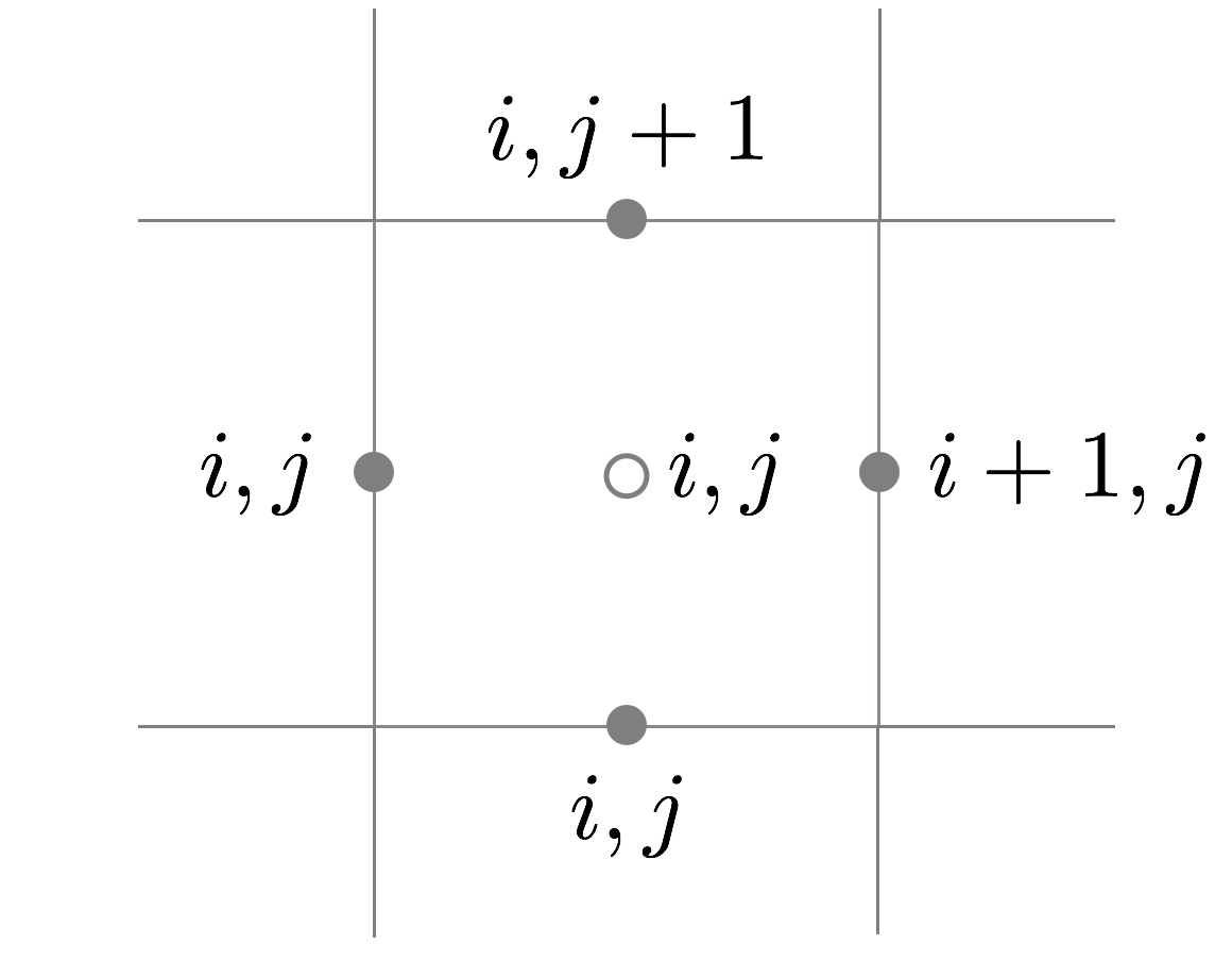
The matlab script by default reads and writes flow fields for use in staggered simulation method. Staggered fields can use different numberings for the velocity. By default the script assumes the numbering
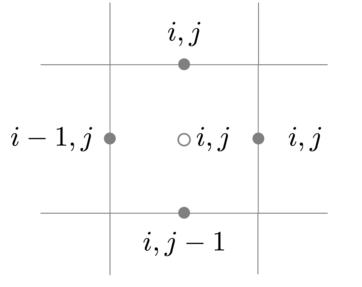
By setting the variable jnumb to 1, an alternative numbering is used.
Sample Fortran code to read and write the generated binary flow files are provided in readwrite.f90.
Higher-order accurate and collocated methods
By default the matlab script generates flow fields for use in a 2nd-order accurate staggered simulation method. However, by making small adjustments the script can also be used to generate flow fields for use in collocated and higher-order accurate methods. The most important adjustment is to make the field divergence-free with respect to the used numerical discretization. This can be done by changing kmod in fourier_tools/makefield.m to
% 2nd-order accurate staggered
kmod = 2i*sin(pi*m/N)/dx; % which is equal to 1i*sin(k*dx/2)/(dx/2)

% 2nd-order accurate collocated
kmod = 1i*sin(2*pi*m/N)/dx;

% 4th-order accurate collocated
kmod = 4/3*1i*sin(2*pi*m/N)/dx - 1/3*1i*sin(4*pi*m/N)/(2*dx);
For a collocated method the calls to fourier_tools/stagtocol.m and fourier_tools/coltostag.m should be removed.
To assure that the divergence check in the code is correct, you could also change the fourier_tools/ifftdivmax.m to the discretization of the divergence used in your code (this will not affect the fields generated by the script, it is just a check).
References
[1] Genevieve Comte-Bellot and Stanley Corrsin. Simple Eulerian time correlation of full-and narrow-band velocity signals in grid-generated, isotropic turbulence. Journal of Fluid Mechanics, 48, pp 273-337 (1971)
[2] Wybe Rozema, Hyun J. Bae, Parviz Moin and Roel Verstappen. Minimum-dissipation models for large-eddy simulation. Physics of Fluids, 27, 085107 (2015)
[3] Dochan Kwak, William C. Reynolds and Joel H. Ferziger. Three-dimensional time dependent computation of turbulent flow. Technical Report, Stanford University (1975)
[4] Hyung Suk Kang, Stuart Chester and Charles Meneveau. Decaying turbulence in an active-grid-generated flow and comparisons with large-eddy simulation. Journal of Fluid Mechanics, 480, pp 129-160 (2003)