The Sound Fourier Transform
Using Fourier Transforms to understand differences in human auditory perception
(The repo with the code & .wav data clip is available on GitHub)
Explore how Fourier transform can help us understand human sounds. Two years ago, the Laurel/Yanny audio clip ignited the internet. Some people hear the clip play as “Laurel” and some hear it as “Yanny”. Several news outlets posted explanations of the different perceptions, and made tools that let you perceive both interpretations. Here I will use Fourier transforms to figure what’s all the fuss about! Fourier transforms are a tool to express physical signals (of space or time) into the frequency space. For now, load the libraries!
import numpy as np
import scipy.io.wavfile as wavfile
import matplotlib.pyplot as plt
# %matplotlib inline
import os
Load the .wav file
I’ll load the Laurel/Yanny audio clip, and process it in several ways that accentuate the “Laurel” or “Yanny” perceptions. It is easy to load an audio file, such as the LaurelYanny.wav file. I also need to keep track of the “sample rate” of the file, which corresponds to the number of datapoints per second
with open("laurel_yanny.wav", 'rb') as file:
    sampleRate, data = wavfile.read(file)
Play the sound by writing the read file into a .wav file.
def writeWavFile(data, filename, sampleRate):
    data1 = (data* 1/np.max(abs(data)) * 32767).astype(np.int16)
    with open(filename + '.wav', 'wb') as f:
        wavfile.write(f, sampleRate, data1)
I only hear “Laurel” – EXCLUSIVELY! You?
Plot the raw signal
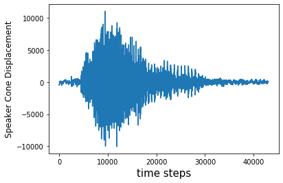
Plot the waveform that this 43,008 point signal array represents.
plt.figure()
plt.plot(data)
recordTime = data.shape[0]/sampleRate # seconds
print("record time is", recordTime, "s")
plt.xlabel('time steps', fontsize = 15)
plt.ylabel('Speaker Cone Displacement', fontsize = 12)
Take the Discrete Fourier Transform
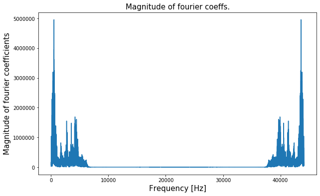
Take the discrete Fourier transform of the signal, and plot the real number corresponding to the magnitude of each coefficient of the Fourier transform. The great thing about taking the Python DFT is that it is implemented using a cool algorithm (FFT) that runs in near linear time (technically \(O(Nlog(N))\)) in the length of the vector (think a single pass efficiency! that’s very good for bulky data).
sp = np.fft.fft(data)
freq = np.fft.fftfreq(n=data.shape[0], d=timestep)
plt.figure(figsize = (10,6))
plt.plot(np.arange(len(sp))/recordTime, abs(sp))
plt.xlabel('Frequency [Hz]', fontsize = 15)
plt.title("Magnitude of fourier coeffs.", fontsize = 15)
plt.ylabel('Magnitude of fourier coefficients', fontsize = 15)
Observations
- Notice the symmetry of the plot of the magnitude of the Fourier coefficients – that is due to the nature of the rows of the Fourier transformation matrix.
- The signal’s Fourier transform has a fairly sparse representation – this plot above is expected because from the plot of previous section, it can be seen that the audio signal is in fact very dense in the temporal space but has some periodicity in it. A typical rule of thumb for signals that are dense in the physical space is that they are sparse in the Fourier space. And vice-versa. Typically, not always
- There is a primary frequency component with the largest Fourier coefficient at frequency<1000Hz.
- There are 4 other key frequency regimes where the Fourier coefficient magnitude peaks. All these peaks are comparable yet smaller than the component with highest corresponding coefficient.
Plot the spectrogram to analyze the energy of signal
The “spectrogram” of the signal illustrates how the amount of high/low frequencies change over the course of the audio clip. Specifically, I’ll chop the signal up into 500-sample long blocks, and compute the Fourier transform for each chunk.
The x axis corresponds tothe index of the chunk, and the y values corresponds to frequencies, and the value at location x, y corresponds to the magnitude of the y\(^{th}\) Fourier coefficient for the x\(^{th}\) chunk. Since frequencies beyond the 80\(^{th}\) Fourier coefficient are too high for humans to hear, the y-axis should just go from 1 to 80.
numChunks = np.floor(data.shape[0]/500).astype(np.int)
A = np.zeros((80, numChunks))
for chunk in range(numChunks):
    start = chunk*500
    end = start+500
    absCoeffs = abs(np.fft.fft(data[start:end]))[0:80].reshape(80,)
    A[:, chunk] = absCoeffs

plt.figure(figsize = (10,8))
plt.imshow(A, cmap = 'hot')
plt.colorbar()
plt.xlabel('Chunk id', fontsize = 15)
plt.ylabel('kth Frequency Component', fontsize = 15)
plt.title('Heatmap of Abs(Fourier Coeffs.)', fontsize = 15)
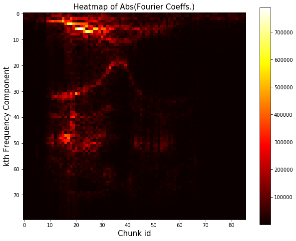
There is for sure some curious structure. Let’s take the log to enhance the contrast
plt.figure(figsize = (10,8))
plt.imshow(np.log(A), cmap = 'hot')
plt.colorbar()
plt.xlabel('Chunk id', fontsize = 15)
plt.ylabel('kth Frequency Component', fontsize = 15)
plt.title('Heatmap of Abs(Fourier Coeffs., log for contrast)', fontsize = 15)
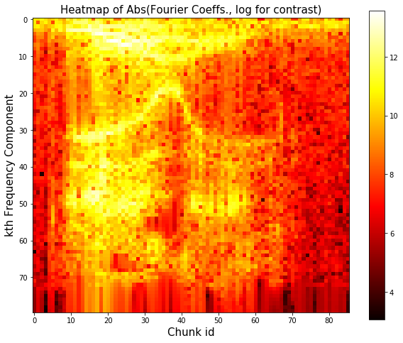
Non monotonic energy transfer trend: Energy is getting transferred from lower to higher frequency with time for “lower” frequency range (freq \(<\) 17th component freq) and the transfer reverses direction after some time (after chunk 40 in particular). Reverse energy transfer observed for frequencies in the 17th-40th band.
Tweaking the signal to achieve pure “Laurel”/”Yanny” sound
Now I will change the signal to sound more like “Laurel” or, more like “Yanny”. To start, I will take the original audio, and try
- zeroing out all “high” frequencies—frequencies above a certain threshold , and
- zeroing out all frequencies below it.
This can be accomplished by multiplying the Fourier transform of the signal by the thresholding function, then taking the inverse Fourier transform. This is what the function below achieves
def thresholding(limit, threshold):
"""
Thresholding function to curb frequencies beyong a threshold
args:
limit: Thresholding Type : "Upper" or "Lower"
-- "Upper" corresponds to zeroing out on the higher frequencies
-- "Lower" corresponds to zeroing out on the lower frequencies
threshold: thresholding frequency
"""
if limit=='Upper':
c1=1
c2=0
elif limit=='Lower':
c1=0
c2=1
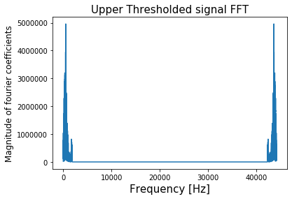
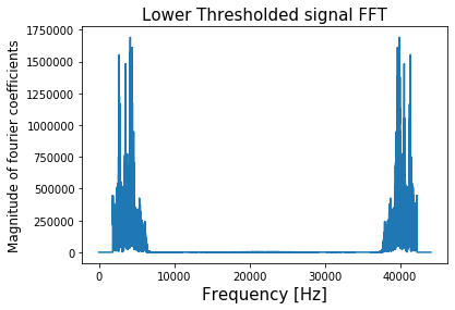
thresholdedFFT = np.hstack((c1*sp[0:threshold],c2*sp[threshold:-threshold], c1*sp[-threshold:])).ravel()
plt.figure()
plt.plot(np.arange(len(sp))/recordTime, abs(thresholdedFFT))
plt.xlabel('Frequency [Hz]', fontsize = 15)
plt.title(limit + " Thresholded signal FFT", fontsize = 15)
plt.ylabel('Magnitude of fourier coefficients', fontsize = 12)
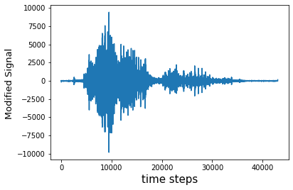
test_o = np.fft.ifft(thresholdedFFT)
# audio signal written to current directory for listening
plt.figure()
plt.plot(test_o)
plt.xlabel('time steps', fontsize = 15)
plt.ylabel('Modified Signal ',fontsize = 13)
fname = 'testing'+limit
writeWavFile(test_o, fname, sampleRate)
Playing around with the threshold value tells me the threshold of around 1850 Hz such that the “low” frequency version sounds like “Laurel” and the “high” frequency version sounds like “Yanny/Yarry”
threshold =  1800
freqThreshold = 1800/recordTime
print(freqThreshold)
thresholding('Upper', threshold)
1845.703125

thresholding('Lower', threshold)
Other ways of bringing out the Laurel or Yanny in the original audio
Keep manually changing the playback by changing the sampling rate and replaying this file
writeWavFile(data, 'playx_testing', np.floor(2*sampleRate).astype(np.int))
Observations
- For very low playbacks of 0.25x-0.45x, I hear some very disturbing and insidious sounds haha!
- At playback of 0.5x – I hear “LOL”
- But I am amazed at what happens at playback of 0.7-0.9 – I hear “Yanny”/”Yarry” exclusively !!
- At orginal playback (1x) and for higher playbacks (>1x), I hear “Laurel” exclusively back again
- And some funny “Laurel” like sound at 2x
Conclusion
Finally we now know that the signatures for sounds that are purely “Laurel”-like haver “lower” frequencies (less than \(\sim\)1850 Hz) and “Yanny” sound has signature in “higher” frequencies (above that threshold). Clearly, from our analysis, we now know that different humans are perceptive to different frequencies. This must be a biological characteristic and needs further looking into! And