Automated Anomaly Detection for Safecast’s Air Quality Sensors
Assisting citizen-science based NPO, Safecast, by automating anomaly detection in air-quality and nuclear-radiation sensors deployed around the globe. This is past volunteer work I carried out in the capacity of a Data Ambassador at DataKind-SF in the hope to help Safecast in its non-profit mission for a more environmentally aware citizenry. Detailed code is hosted on Github.
Introduction
Safecast is a citizen science organization which supports collection of radiation and air quality data around the world with citizens as the primary leads for data acquisition. For data acquisition, Safecast provides citizens and also independently deploys sensors at various locations around the globe. There are multiple device types, and for each device, there are multiple deployments. The data for radiation levels and air quality (AQ measured as Particulate Matter (1, 2.5, and 10)) has been supplied to DataKind. The acquired data has anomalies which may be due to realistic environmental conditions, human error, hardware and/or firmware issues at the sensor level, or, data transmission issues. Detection of such anomalies would enable Safecast to detect which sensors could be malfunctioning and which need to be repaired/replaced in a timely fashion. Timely attention to malfunctional sensors will also ensure that invalid data is not stored thereby saving cloud storage requirements and costs. Detecting anomalies that could be tied to one or more of the issues listed above will help Safecast monitor the quality of citizen-based measurements while also monitoring reliability and issues with sensor deployments.
Overview of Data Source and Analysis Framework
I will analyze historical time series of radiation and air-quality data and develop strategies to enlist anomalous events for data from the Solarcast devices. Solarcast devices are static panels with 36 deployments around the world. Many of the devices have been functional since 2017. These devices, which are GPS enabled, house 2 radiation sensors, 3 air-quality sensors, and sensors for measuring relative humidity and panel temperature. The devices log data at unequal intervals but a representative frequency of logging would be around 10 minutes. All of Safecast’s data is publicly hosted on their website and the reader should feel free to explore data from other devices (other than the Solarcast devices) such as the Pointcasts, bGeige-nanos, Solarcast-nanos etc.
Here I will demonstrate how we can leverage a combination of complex data lookups, data interpretation and simple-meaningful algorithms to identify anomalies in a given dataset. The language I have used for data cleaning and analysis is Python (in particular, the pandas library will be my primary workhorse) but ANSI SQL will work just fine too. To quickly generate interactive visualizations for heavy volume data, I am using the holoviews library powered by bokeh.
Setting the Objective: Metrics and The Unsupervised Setting
Going forward, note that the data itself will be unlabelled, i.e., the data is unaware of the characteristics of anomalous events. The objective is to automate detection of anomalies in the radiation and air-quality data as measured by a variety of sensors in an unsupervised setting. Note that from a data science perspective, the task of detection is descriptive since the data is unlabelled. This is to say that there are no causal or predictive components to the task of anomaly detection. The anomalies that will be tagged as alerts in this way can be result of both environmental factors (false positive alerts) as well as sensor degradation (true positive alerts) such as accumulation of dust for instance. But since there is no way for us to know what the cause of an anomaly might be, I will go ahead and take the more conservative approach of tagging any spurious event as an alert (anomaly). This is conservative since we want to raise as many alerts as we can in the absence of causal labels so that we never miss on events that were because of faulty sensors but went undetected. In other words, it’s OK to tag spurious events that are realistically caused by the surrounding environment as alerts.
Data Payloads
Engineers at Safecast have enabled pulling the data for all Solarcast devices through automated scripts such that we have a series of .csv files for each day with data logs for each of the devices since they have been logging data. The key fields of interest are
- The air quality indices as measured by the sensors in the Solarcast panels: these correspond to PM1.0, PM2.5, and PM10.0 measurements. These are respectively stored as
pms_pm01_0,pms_pm02_5andpms_pm10_0fields. PM1.0 is proportional to the concentration of particulate matter that is 1.0 micrometer or less in size. Similarly for PM2.5 and PM10.0. Air quality data is visualized below for one particular device. Note that this data is already “cleaned” with heuristics as described in the section below.
Figure: Sample Air Quality Index (AQI) time-series visualized using the holoviews library in python. AQI is measured as PM’x’ for one of the 36 solarcast devices. ‘x’ here can be 1.0, 2.5, or 10.0. The plot is an interactive one and the widgets to the right of it will allow you to zoom, pan and explore the visual more fully.
Key Insight: Notice how the PM values are correlated at any given instance of time. This makes sense also because if the overall AQ is good, it is reasonable to expect that particles of all sizes are low in concentration. This correlation is also due to the fact that PM2.5 concentration is by definition a part of the PM10.0 measurement since particles of size 2.5 micrometer or less are also less than 10 micrometer in size. The relation PM1.0<PM2.5<PM10.0 should always hold at any location and time. Below is a plot of the Pearson Correlation coefficient to see how well any two of the 3 AQI indices are correlated. A correlation coefficient of 1 denotes perfect correlation and tells that the time series in question (here PM1.0 and PM10.0) go hand in hand, i.e. an increase in one corresponds to increase in the other. This is typically what can be seen in the figure below.
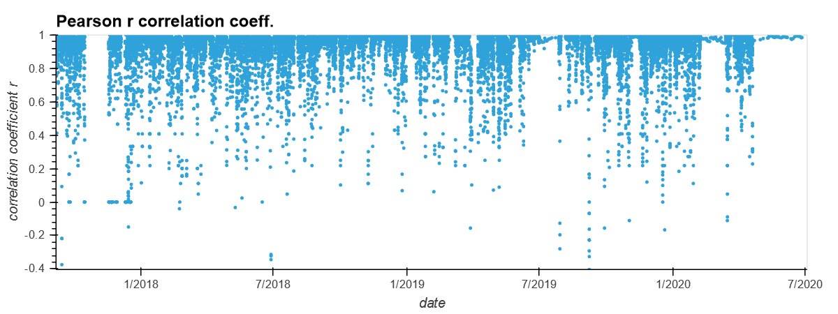 Figure: The Pearson Correlation coefficient between PM10 and PM1 for the device discussed in this post. Notice how the correlation coefficient is almost always ~1
- The next important payload of the data is the nuclear radiation measurements in the units of ‘CPM’ or Counts per Minute. These are measured by 2 different sensors and stored as
lnd_7318candlnd_7318ufields. The difference between the two lies in the fact that the two sensors measure radiation in different ways.
Figure: Sample radiation measurement (in CPM or counts-per-minute) time-series visualized using the holoviews library in python. The widgets to the right of it will allow you to zoom, pan and explore the visual more fully.
- The
devicepayload. This is a unique identifier for each device. - The timestamp for when the data was measured. This is stored in the
when_capturedfield. - The environmental relative humidity as stored in the
env_humidfield. - The panel temperature as stored in the
env_tempfield.
Overview of the Data Cleaning Heuristics
-
Prior to analyzing data, raw data will have to be cleaned to make it ready for analysis. I will bypass the ETL process for this post but feel free to reach out if you’re interested.
-
The next step in the pipeline is the data cleaning step where I address issues of consistency, validity and accuracy for the raw data to make it usable. The output of this step is a master data file in the
.csvformat (hosted here) which has data records for each device for each time-stamp since they have been deployed in field. Here I am listing known issues in the data and how I have addressed these issues. For the implementation of these heuristics, see the code here. Feel free to reach out to me if you have any questions.- Consistency: Format of the various entries for a payload are not consistent in the raw dataset. For instance, the
pms_pm01_0data values are not consistently stored as floats: there are some mixed data types such as strings too. Similarly, for the radiation data. I use code such as:df['pms_pm01_0'] = df['pms_pm01_0'].astype(str).str.replace(',', '').astype(float)to make the record data types consistent. - Validity: Environmental humidity, recorded as relative humidity (RH) here, is by definition bounded between 0 and 100. There are bugs in the sensor which lead the results to be out of bound RH values. I replace those humidity values with
NaNs. - Accuracy: There are multiple different records for a device which are all time-stamped with the same value of
when_capturedfield. This is of course unrealistic as there cannot be two measurements at the same time. The reason there could be such values is because of data transmission and firmware issues (see here). Since there is no way to trace back (after speaking with Safecast) which one or more of these is the correct record if at all, these data records only add to ambiguity. So I have discarded such records. - Miscellaneous corrections: There are other known issues with the sensor firmware and the data transmission to cloud. Knowledge of these has enabled me to further clean the data. These are discussed in the
data_cleaner.pycode file.
- Consistency: Format of the various entries for a payload are not consistent in the raw dataset. For instance, the
Automating Anomaly Detection For Unlabelled Data
The data is cleaned and the output is stored in a master .csv file. Now I will use 2 key heuristics to find anomalies in the AQ data. The output of this pipeline will be a list of all records in the data that are anomalous based on a “normalized-severity-score” score for each event. The score is a numeric index whose value is proportional to how severe I find the anomaly is. Any event whose score surpasses a pre-specified “threshold” (which can take multiple forms) will qualify for an anomaly that can alert the user – Safecast in this case.
Methods for finding outliers
Approach 1: Day vs. Night Median AQ Disparity
One expects that the AQ would typically be better during the night time than during the preceding day time. This is also corroborated from observations as seen in the figure below. This is of course only a heuristic (a reasonable one) and not a hard-bound rule. Nevertheless, if the night time median AQ is observed to be greater than the preceding day’s median AQ, then it can be reason for concern for why that happened. It could be a result of environmental degradation at night time. This could be attributable to for instance a nocturnally operated factory close to the sensor for instance which might be ejecting smoke. It could also be due to a sudden splurge in traffic due to a nearby concert. Or even firecrackers. But it could also be the case that the sensor is malfunctioning. The bet is to detect the malfunctional behavior and it’s OK if there are false positive anomalies (ones that are due to the environment but are tagged as sensor anomalies nevertheless).
Figure: The PM10 data is visualized with differently colored data points for the nocturnal records and the day-time records. More often than not, the day-time PM values are higher than the night-time ones. The black dots denote nights where the median PM10 is more than the preceding day’s median PM10.
To define a representative value of the PM for the night and for the day, I take median of the data values. Day-time is defined as the period from 6am to 6pm on a particular date. Night-time is defined as the period between 6pm and the following date’s 6am for the figure above. These day_start (6am) and day_end (6pm) hours are hyperparameters of the model. In addition, min_rec is another hyperparameter which is the minimum number of records in the daytime and night-time that need to be present for a 24hour period under study for a median to be well defined. Below is the code snippet that evaluates the day and night median PMs.
medians_sf = {}
# field is pms_pm10_0
# report dates and devices as anomalies when the date's night time median is larger than day time median
# -- works for PMS only -- not for radiation
for curr_date in dates:
# get the median for daytime value for the current date
day_mask = (sf.get_group(curr_date).hod >=day_start) & (sf.get_group(curr_date).hod < day_end)
day_vals= sf.get_group(curr_date)[field][day_mask]
# only evaluate a meaningful median if there are more than min_rec records in the day
if len(day_vals) >= min_rec:
day_median = day_vals.median()
else:
day_median = np.nan
# get the median nighttime value for the current date
night_mask_curr = sf.get_group(curr_date).hod >= day_end
night_vals_curr = sf.get_group(curr_date)[field][night_mask_curr]
night_vals_next = []
# if the next consecutive date exists in the time series, then use the records until 6am on that date
# as they correspond to the "night" of the current date (`curr_date`)
if curr_date + datetime.timedelta(1) in dates:
night_mask_next = sf.get_group(curr_date + datetime.timedelta(1)).hod < day_start
night_vals_next = sf.get_group(curr_date+ datetime.timedelta(1))[field][night_mask_next]
night_vals = night_vals_curr.append(night_vals_next)
# only evaluate a meaningful median if there are more than min_rec records in the night
if len(night_vals) >= min_rec:
night_median = night_vals.median()
else:
night_median = np.nan
# store the medians in a double valued list for the curr_date key in dict `medians_sf`
medians_sf[curr_date] = [day_median, night_median]
The hyperparameters discussed above: day_start, day_end and min_rec need to be tuned manually based on the desired response. The figure above shows the day and night values as well as indicates the locations with black dots that need attention – i.e., where the night-time records’ median is more than the day’s median.
Scoring: I define the severity of the anomaly with a score as
`temp['normalized_severity_score'].append((lst[1]-lst[0] + 1)/(lst[0]+1))`
This represents the difference between the night-time median PMx (lst[1]) and the day-time median (lst[0]) as a fraction of the day-time median. The +1 in the numerator and denominator is the Laplace smoothing method to ensure that the denominator is never 0.*
Key Insight: The key takeaway is that we are able to catch a decent number of events as anomalies and associate the severity score with each. We would suspect these might be due to sensor issues since we know that night-time AQ should be on average better than the preceding day’s AQ. Notice that the same heuristic does not hold good for radiation measurements since there is little reason or evidence to show that the night-day disparity between radiation measurements follow a trend.
Approach 2: n-Standard Deviations away from Rolling-median
It is also apparent from the data that there are spurious events or outliers in the time series that appear to be sudden jumps or spikes in an otherwise relatively low variance time-series. I would now like to tag these outliers as anomalies. But to find out what is an outlier, I first need to identify a certain type of a “normal” trend of the data. To capture this normal, I adopt the method of taking the running (or rolling) median of the time series (note that I chose running median instead of the running mean to avoid the normal from being severely affected by outliers in a time window of interest). The idea here is to choose a window of contiguous timestamps and calculate the median PM in that window. The evaluation starts at the beginning of the time series and the window is then slided by one record to the right each time to progress in the time series. The assumption that the median is a decent approximation for the representative AQ in that time window is reasonable since one does not expect the AQ to change drastically within a short window. Of course, window size is a hyperparameter to be tuned by manual inspection of what works for a group of devices.
After identifying this underlying normal, an event that does not lie within +/- n-Standard deviations of this normal is tagged as an anomalous event. The code snippet below is used to evaluate the rolling median and the +/- n-Standard deviation bounds. Note that n is also a hyperparameter. Another hidden hyperparameter is the min_period. This is the minimum number of records in a window that are required for a median to be calculated and therefore be meaningful. This is necessary because as you will notice from the figure below, there are a lot of observations that are in fact missing in the cleaned version of the data.
deviceFilter = df['device'] == device
rollingMedian = df[deviceFilter][field].rolling(window, min_periods=min_period).median()
rollingStdev = df[deviceFilter][field].rolling(window, min_periods=min_period).std()
upper = rollingMedian + (rollingStdev * numStd)
lower = rollingMedian - (rollingStdev * numStd)
# visualize
x = pd.to_datetime(df[deviceFilter]['when_captured']).values # timestamps for the x axis
line1 = hv.Scatter((x,df[deviceFilter][field]), label='data').opts(width=700, ylabel = field)
line1Median = hv.Curve((x, rollingMedian), label='Median').opts(width=700, color='red', xlabel = 'date')
line1Upper = hv.Curve((x, upper), label='Median+ 3.stdev').opts(width=700, color='blue')
line1Lower = hv.Curve((x, lower), label='Median- 3.stdev').opts(width=700, color='blue')
# holoviews visual generation
overlay = line1Upper * line1Median * line1 * line1Lower
overlay.opts(title="device: "+str(device))
Figure: The PM10 data is visualized along with the rolling median and the +/- 3 standard deviation bounds. The model works well for most devices including this one. Any event that lies outside the +/- 3 standard deviation bounds is tagged as an anomaly. 3 hyperparameters of the model are : window size, n (here = 3), min_period (here chosen to be half the window size).
The model is not perfect as can be seen from the figure above but is seen to perform overall very well in capturing outliers for most devices. The key is to carefully tune the 3 hyperparameters.
Scoring: I define the normalized score for an anomaly as
`temp['normalized_severity_score'] = (temp[field]-temp['rollingMedian'])/(numStd*temp['rollingStdev'])`
This is the deviation away from the median in units of the standard deviation at that point.
A similar approach is used for detecting outlier events in the radiation data as well. Below is an interactive illustration of the rolling median for the radiation data and the +/- 3 standard deviation bounds.
Figure: The radiation data from one of the sensors is visualized along with the rolling median and the +/- 3 standard deviation bounds. The model is akin to the corresponding PM10 data visualized above. Notice how well the 3 standard-deviation bounds are able to capture the range of measurements for the most part. The outliers are then tagged as anomalies.
Key insight: Using a locally calculated median as the “normal trend”, and bounds on values of the quantity of interest using the locally calculated standard deviation, we are able to capture more anomalies which leaves us in good shape.
Miscellaneous approaches
There are some additional heuristics that were incorporated in the anomaly detection procedure. These are also captured in the anomaly_detector.py file.
- Trend of PM measurements: As discussed before, the PM measurements at any space and time location must be such that PM1.0<PM2.5<PM10.0. There are measurements in the dataset which don’t follow this and have been flagged as anomalies with severity score as 1. This is a self-starter function which does not require any hyperparameter tuning.
- Large gap between consecutive measurments: It is also common that the dataset being used has gaps between consecutive measurements. I flag events for which the next measurement is available after
day_gapnumber of days (defaults to 2 days) as anomlaous. Note that if the input data is pre-cleaned such as after applying the cleaning heuristics, then some of these flags will be because records were discarded in the cleaning pipeline. But there will be other records which will be because the the sensor in fact does not log any data forday_gapdays (can be fractional duration in the units of days). This could hint at which sensors might be failing.day_gapis the only hyperparameter that needs tuning for this function again based on how often Safecast would like to receive sensor alerts.
Conclusions & Outlook
- We note that using two heuristics: first, anomaly detection based on night-day disparity of air-quality measurements and second, deviations away from the rolling median, we are able to capture most if not all of the anomalies in the data that could be attributable to sensor malfunction. For radiaton data, only the latter technique would work.
- This is ongoing work, and a lot more needs to be done. In the future, I would be interested in exploring if the time-series can be decomposed into a “seasonality” part, a “trend” part and a “residual” part.
- An important takeaway is that data cleaning can take up to 70% of the actual exploration! Real world data is not clean and as a data scientist, I take pride in having to dig into it and clean it! This is fun!
- Finally notice that simple techniques such as above can be good for solving a descriptive challenge such as this one. We have not invoked machine learning or other AI methods here for learning of hyperparameters! The goodness of our approach remains to be quantified since this is an unsupervised setting, so Safecast’s feedback will be useful here as they are the domain experts.