t_SystemSimulate

t_IntroductionISET.m
Initialize ISET
Initialize some parameters
Scene
Optics
Sensor
Set these sensor properties
Image Processor
END

t_IntroductionISET.m

This script illustrates how to create the full array of elements that make up the image simulation steps.

% Use t_"TAB KEY" to see the list of tutorials
% Use s_"TAB KEY" to see the list of ISET scripts.
%
% See also: t_IntroductionScene.m and t_IntroductionOI.m
%
% To learn more about a particular function, type "help function" as in "help sensorCreate".
%
% Copyright ImagEval Consultants, LLC, 2010.

Initialize ISET

ieInit

Initialize some parameters

% In this example, wavelengths range between 400 and 710 nm, sampled every
% 5 nm. It is also possible to expand the range to include wavelengths in
% the near infrared (NIR) range. Of course, this would only make sense if your
% imaging sensor has sensitivity in the NIR range.
wave = 400:5:710;

Scene

Create a radiometric description of the scene. There are several ways to create a scene. see scripts/scenes for more information about scenes

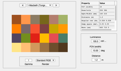
One is to use the sceneCreate function. In the example below, we create a scene of the Macbeth Color Checker illuminated with a tungsten light For a complete list of the types of synthetic scenes type "help sceneCreate"

A second method for creating a scene is to read data from a file. ISET includes a few multispectral scenes as part of the distribution. These can be found in the data/image/multispectral directory You can also select the file (or many other files) using the command: fullFileName = vcSelectImage;

see s_sceneFromMultispectral.m, s_sceneFromRGB.m

patchSize = 64;
scene = sceneCreate('macbeth tungsten',patchSize,wave);

% It is often useful to visualize the data in the scene window
sceneWindow(scene);

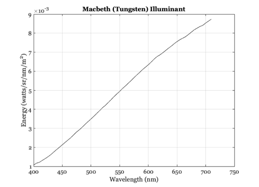
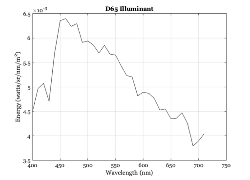
Each scene has a stored illuminant.

scenePlot(scene,'illuminant energy roi');

No ROI needed unless spatial spectral illluminant

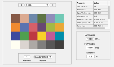
It is possible to change the scene illuminant

scene = sceneAdjustIlluminant(scene,'D65.mat');
scene = sceneSet(scene,'name','D65'); % Set the scene name
sceneWindow(scene);

Once the scene is loaded, you can adjust different properties using the sceneSet command. Here we adjust the scene mean luminance and field of view.

scenePlot(scene,'illuminant energy roi');
scene = sceneAdjustLuminance(scene,200);  % Candelas/m2
scene = sceneSet(scene,'fov',26.5);       % Set the scene horizontal field of view
scene = sceneInterpolateW(scene,wave,1);  % Resample, preserve luminance
% sceneWindow(scene); % if you want to view the change in the GUI window

No ROI needed unless spatial spectral illluminant

Optics

see t_IntroductionOI.m

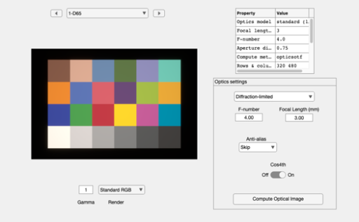
The next step in the system simulation is to specify the optical image formation process. The optical image is an important structure, like the scene structure. We adjust the properties of optical image formation using the oiSet and oiGet routines.

ISET has several optics models that you can experiment with. These include shift-invariant optics, in which there is a different shift-invariant pointspread function for each wavelength, and a ray-trace method, in which we read in data from Zemax and create a shift-variant set of pointspread functions along with a geometric distortion function.

The simplest is method of creating an optical image is to use the diffraction-limited lens model. To create a diffraction-limited optics with an f# of 4, you can call these functions

oi = oiCreate;

optics = oiGet(oi,'optics');

oi = oiSet(oi,'optics fnumber',4);
% optics = opticsSet(optics,'fnumber',4);

% In this example we set the properties of the optics to include cos4th
% falloff for the off axis vignetting of the imaging lens, and we set the
% lens focal length to 3 mm.
oi = oiSet(oi,'optics off axis method','cos4th');
oi = oiSet(oi,'optics focal length',3e-3);     % from lens calibration software

% We use the scene structure and the optical image structure to update the
% irradiance.
oi = oiCompute(oi,scene);

% We save the optical image structure and bring up the optical image
% window.
oiWindow(oi);

% From the window you can see a wide range of options. These include
% insertion of a birefringent anti-aliasing filter, turning off cos4th
% image fall-off, adjusting the lens properties, and so forth.
%
% You can read more about the optics models by typing "doc opticsGet".
%

Sensor

The irradiance is then captured by a simulated sensor, resulting in an array of output voltages. There are a very large number of sensor parameters. Here we illustrate the process of creating a simple Bayer-gbrg sensor and setting a few of its basic properties.

To create the sensor structure, we call

sensor = sensorCreate('bayer (gbrg)');

% We set the sensor properties using sensorSet and sensorGet routines.
%
% Just as the optical irradiance gives a special status to the optics, the
% sensor gives a special status to the pixel.  In this section we define
% the key pixel and sensor properties, and we then put the sensor and pixel
% back together.

% To get the pixel structure from the sensor we use:
pixel =  sensorGet(sensor,'pixel');

% Here are some of the key pixel properties
voltageSwing   = 1.15;  % Volts
wellCapacity   = 9000;  % Electrons
conversiongain = voltageSwing/wellCapacity;
fillfactor     = 0.45;       % A fraction of the pixel area
pixelSize      = 2.2*1e-6;   % Meters
darkvoltage    = 1e-005;     % Volts/sec
readnoise      = 0.00096;    % Volts

% We set these properties here
pixel = pixelSet(pixel,'size',[pixelSize pixelSize]);
pixel = pixelSet(pixel,'conversiongain', conversiongain);
pixel = pixelSet(pixel,'voltageswing',voltageSwing);
pixel = pixelSet(pixel,'darkvoltage',darkvoltage) ;
pixel = pixelSet(pixel,'readnoisevolts',readnoise);

%  Now we set some general sensor properties
% exposureDuration = 0.030; % commented because we set autoexposure
dsnu =  0.0010;           % Volts (dark signal non-uniformity)
prnu = 0.2218;            % Percent (ranging between 0 and 100) photodetector response non-uniformity
analogGain   = 1;         % Used to adjust ISO speed
analogOffset = 0;         % Used to account for sensor black level
rows = 466;               % number of pixels in a row
cols = 642;               % number of pixels in a column

Fill factor may have changed. You can use: size same fill factor

Set these sensor properties

sensor = sensorSet(sensor,'exposuretime',exposureDuration,method); % commented because we set autoexposure

sensorSet(sensor,'autoExposure',1,'default');
sensor = sensorSet(sensor,'rows',rows);
sensor = sensorSet(sensor,'cols',cols);
sensor = sensorSet(sensor,'dsnu level',dsnu);
sensor = sensorSet(sensor,'prnu level',prnu);
sensor = sensorSet(sensor,'analog Gain',analogGain);
sensor = sensorSet(sensor,'analog Offset',analogOffset);

% Stuff the pixel back into the sensor structure
sensor = sensorSet(sensor,'pixel',pixel);
sensor = pixelCenterFillPD(sensor,fillfactor);

% It is also possible to replace the spectral quantum efficiency curves of
% the sensor with those from a calibrated camera.  We include the
% calibration data from a very nice Nikon D100 camera as part of ISET.
% To load those data we first determine the wavelength samples for this sensor.
wave = sensorGet(sensor,'wave');

% Then we load the calibration data and attach them to the sensor structure
fullFileName = fullfile(isetRootPath,'data','sensor','colorfilters','nikon','NikonD100.mat');
[data,filterNames] = ieReadColorFilter(wave,fullFileName);
sensor = sensorSet(sensor,'filter spectra',data);
sensor = sensorSet(sensor,'filter names',filterNames);
sensor = sensorSet(sensor,'Name','Camera-Simulation');

% We are now ready to compute the sensor image
sensor = sensorCompute(sensor,oi);

% We can view sensor image in the GUI.  Note that the image that comes up
% shows the color of each pixel in the sensor mosaic. Also, please be aware
% that the Matlab rendering algorithm often introduces unwanted artifacts
% into the display window.  You can resize the window to eliminate these.
% You can also set the display gamma function to brighten the appearance in
% the edit box at the lower left of the window.
sensorWindow(sensor);

% There are a variety of ways to quantify these data in the pulldown menus.
% Also, you can view the individual pixel data either by zooming on the
% image (Edit | Zoom) or by bringing the image viewer tool (Edit | Viewer).
%
% Type 'help iexL2ColorFilter' to find out how to convert data from an
% Excel Spread Sheet to an ISET color filter file or a spectral file/
%
% ISET includes a wide array of options for selecting color filters
% fill-factors, infrared blocking filters, adjusting pixel properties,
% color filter array patterns, and exposure modes.

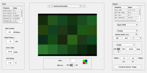
Image Processor

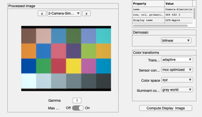
The sensor array is demosaiced, color-balanced, and rendered on a display The image processing pipeline is managed by the fourth principal ISET structure, the virtual camera image (vci). This structure allows the user to set a variety of image processing methods, including demosaicking and color balancing.

vci = ipCreate;

% The routines for setting and getting image processing parameters are
% ipGet and ipSet.
%
vci = ipSet(vci,'name','Unbalanced');
vci = ipSet(vci,'scaledisplay',1);

% The default properties use bilinear demosaicking, no color conversion or
% balancing.  The sensor RGB values are simply set to the display RGB
% values.
vci = ipCompute(vci,sensor);

% As in the other cases, we can bring up a window to view the processed
% data, this time a full RGB image.
ipWindow(vci);

% You can experiment by changing the processing parameters in many ways,
% such as:
vci2 = ipSet(vci,'name','More Balanced');
vci2 = ipSet(vci2,'internalCS','XYZ');
vci2 = ipSet(vci2,'conversion method sensor','MCC Optimized');
vci2 = ipSet(vci2,'illuminant correction method','Gray World');

% With these parameters, the colors will appear to be more accurate
vci2 = ipCompute(vci2,sensor);

ipWindow(vci2);

% Again, this window offers the opportunity to perform many parameter
% changes and to evaluate certain metric properties of the current system.
% Try the pulldown menu item (Analyze | Create Slanted Bar) and then run
% the pulldown menu (Analyze | ISO12233) to obtain a spatial frequency
% response function for the slanted bar image in the ISO standard.

Contents