t_Simulate4Channel.m
Simulate a 4-channel sensor and render the data
The script begins by creating a full spectral scene. Then the scene radiance data are passed through the optics to create an irradiance image at the sensor surface.
A 4-channel sensor is created with filters containing Gaussian transmittance. The sensor catch is simulated, and the 4-channel data are then rendered.
Key functions: sensorColorFilter
To learn more about a particular function, type "help function" as in "help sensorCreate".
Copyright ImagEval Consultants, LLC, 2010.
Contents
Introduction
To see a more elaborate script that creates scenes and optical images, please review s_SimulateSystem. Here, we just accept the default scene, optical image and focus on creating the 4 channel sensor.
ieInit
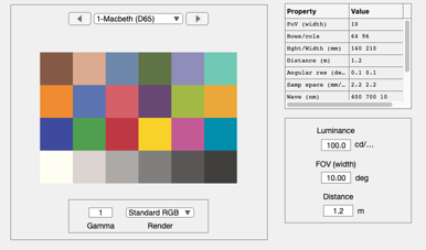
SCENE
scene = sceneCreate;
wave  = sceneGet(scene,'wave');

% It is often useful to visualize the data in the scene window
sceneWindow(scene);

% When the window appears, you can scale the window size and adjust the
% font size as well (Edit | Change Font Size). There are many other options
% in the pull down menus for cropping, transposing, and measuring scene
% properties.
%
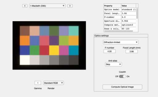
OPTICS
oi = oiCreate;
oi = oiCompute(oi,scene);
oiWindow(oi);
SENSOR
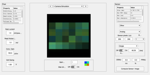
% Create a set of color filters with Gaussian spectral transmittances
cfType = 'gaussian';
cPos   = 450:50:600; width = ones(size(cPos))*25;
d = struct;
d.data = sensorColorFilter(cfType,wave, cPos, width);
d.filterNames = {'b','g','y','r'};
d.comment     = 'Four color simulation for s_Simulate4Channel.m';
d.wavelength  = wave;

% Save them in a tmpFilter file
% filterFile = fullfile(pwd,'tmpFilter.mat');
% ieSaveColorFilter(d,filterFile)

% How the filters are positioned in the 2x2 block.
filterOrder = [1 2 ; 3 4];
pixel = pixelCreate;

% Initialize the sensor structure.  The spectrum is set to match the
% pixel.spectrum entry.
% sensor = sensorCreate('Custom', pixel, filterOrder, filterFile);
sensor = sensorCreate('Custom', pixel, filterOrder, d);
% delete(filterFile);  % Delete to keep the directory clean

sensor = sensorSet(sensor,'fov',sceneGet(scene,'fov')*1.1,oi);

sensor = sensorSet(sensor,'Name','Camera-Simulation');

% Now load the IR filter
fullFileName = fullfile(isetRootPath,'data','sensor','irfilters','irFilter_schott.mat');
irData = ieReadColorFilter(wave,fullFileName);
sensor = sensorSet(sensor,'irFilter',irData);

% We are now ready to compute the sensor image
sensor = sensorCompute(sensor,oi);

% We can view sensor image in the GUI.  Note that the image that comes up
% shows the color of each pixel in the sensor mosaic. Also, please be aware
% that
%  * The Matlab rendering algorithm often introduces unwanted artifacts
% into the display window.  You can resize the window to eliminate these.
%  * You can also set the display gamma function to brighten the appearance
% in the edit box at the lower left of the window.
sensorWindow(sensor);

% There are a variety of ways to quantify these data in the pulldown menus.
% Also, you can view the individual pixel data either by zooming on the
% image (Edit | Zoom) or by bringing the image viewer tool (Edit | Viewer).
%
% Type 'help iexL2ColorFilter' to find out how to convert data from an
% Excel Spread Sheet to an ISET color filter file or a spectral file/
%
% ISET includes a wide array of options for selecting color filters
% fill-factors, infrared blocking filters, adjusting pixel properties,
% color filter array patterns, and exposure modes.
PROCESSOR
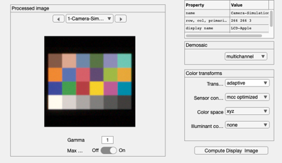
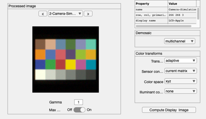
The image processing pipeline is managed by the fourth principal ISET structure, the virtual camera image (vci). This structure allows the user to set a variety of image processing methods, including demosaicking and color balancing
vci = ipCreate;
vci = ipSet(vci,'name','No Balance');
vci = ipSet(vci,'scale display',1);
vci = ipSet(vci,'demosaic method','multichannel');
vci = ipSet(vci,'conversion method sensor ','MCC Optimized');
vci = ipSet(vci,'internal Color Space','XYZ');

vci = ipSet(vci,'correction method illuminant','None');

% The default properties use bilinear demosaicking, no color conversion or
% balancing.  The sensor RGB values are simply set to the display RGB
% values.
vci = ipCompute(vci,sensor);

% This shouldn't be here ... but the 4 channel processing isn't right yet
o = ipGet(vci,'result'); o = o/max(o(:)); vci = ipSet(vci,'result',o);

% As in the other cases, we can bring up a window to view the processed
% data, this time a full RGB image.
ipWindow(vci);
Sensor conversion
% In the sensor window we used the pulldown under
% Analyze | Color | Sensor Conversion Matrix
% to find an optimal transform matrix for the MCC
m = [...
    -0.0528   -0.2091    1.5196
    0.0050    0.3319   -0.0801
    -0.9505    1.0048   -0.0823
    2.4197   -0.1467   -0.0339
    ];
vci = ipSet(vci,'conversion transform sensor',m);

% We set  the other transforms to the identity, so that the product of all
% the transforms is just the one above.
vci = ipSet(vci,'illuminant correction transform',eye(3,3));
vci = ipSet(vci,'ics2Display Transform',eye(3,3));

% We set the vci to not ask any questions, just use the current matrices.
vci = ipSet(vci,'conversion method sensor','current matrix');

% Compute and show.
vci = ipCompute(vci,sensor);
ieAddObject(vci); ipWindow
ans =

  ipWindow_App with properties:

                        figure1: [1×1 Figure]
                       menuFile: [1×1 Menu]
                   menuFileLoad: [1×1 Menu]
           menuFileSaveProcData: [1×1 Menu]
              menuFileLoadImage: [1×1 Menu]
                   menuFileSave: [1×1 Menu]
                menuFileRefresh: [1×1 Menu]
                  menuFileClose: [1×1 Menu]
                       menuEdit: [1×1 Menu]
                   menuEditName: [1×1 Menu]
                 menuEditCreate: [1×1 Menu]
              menuEditCopyImage: [1×1 Menu]
                 menuEditDelete: [1×1 Menu]
             menuEditDeleteSome: [1×1 Menu]
                 menuImageWhite: [1×1 Menu]
             menuEditResetWhite: [1×1 Menu]
             menuScaleChooseMax: [1×1 Menu]
               menuScaleDisplay: [1×1 Menu]
               menuEditFontSize: [1×1 Menu]
           menuEditClearMessage: [1×1 Menu]
                 menuEditViewer: [1×1 Menu]
                       menuPlot: [1×1 Menu]
               menuPlImTrueSize: [1×1 Menu]
               multipleImageRGB: [1×1 Menu]
                menuPlotDisplay: [1×1 Menu]
                 plotDisplaySPD: [1×1 Menu]
                      plotGamut: [1×1 Menu]
    plotColorProcessingMatrices: [1×1 Menu]
                 plotMCCOverOff: [1×1 Menu]
                    menuDisplay: [1×1 Menu]
                    menuReadSPD: [1×1 Menu]
              menuDisplayWindow: [1×1 Menu]
               menuDisplayViewD: [1×1 Menu]
                    menuAnalyze: [1×1 Menu]
                    menuAnColor: [1×1 Menu]
                      menuAnROI: [1×1 Menu]
                      menuAnLum: [1×1 Menu]
                    menuAnChrom: [1×1 Menu]
                 menuAnColorLAB: [1×1 Menu]
                      menuAnLUV: [1×1 Menu]
                    menuRGBHist: [1×1 Menu]
                  menuAnROIvSNR: [1×1 Menu]
          chartClearcornersMenu: [1×1 Menu]
                        MCCMenu: [1×1 Menu]
             LuminancenoiseMenu: [1×1 Menu]
           ColormetricssRGBMenu: [1×1 Menu]
           VisualcompareD65Menu: [1×1 Menu]
                     menuAnLine: [1×1 Menu]
                    menuAnLineH: [1×1 Menu]
                    menuAnLineV: [1×1 Menu]
            menuAnalyzeCreateSB: [1×1 Menu]
            menuAnalyzeISO12233: [1×1 Menu]
              menuMetricsWindow: [1×1 Menu]
        menuAnComputeFromSensor: [1×1 Menu]
              menuComputeFromOI: [1×1 Menu]
         menuAnComputeFromScene: [1×1 Menu]
                       menuHelp: [1×1 Menu]
        menuHelpProcessorOnline: [1×1 Menu]
              menuHelpMetricsPG: [1×1 Menu]
             menuHelpISETOnline: [1×1 Menu]
               menuHelpAppNotes: [1×1 Menu]
                     btnCompute: [1×1 Button]
                  DemosaicPanel: [1×1 Panel]
                    popDemosaic: [1×1 DropDown]
           ColortransformsPanel: [1×1 Panel]
                      txtSensor: [1×1 Label]
                  txtIlluminant: [1×1 Label]
                     popBalance: [1×1 DropDown]
                         txtICS: [1×1 Label]
                  popColorSpace: [1×1 DropDown]
                      txtMethod: [1×1 Label]
            popColorConversionM: [1×1 DropDown]
                   popTransform: [1×1 DropDown]
                        ipTable: [1×1 Table]
            ProcessedimagePanel: [1×1 Panel]
                MaxbrightSwitch: [1×1 Switch]
           MaxbrightSwitchLabel: [1×1 Label]
                     txtMessage: [1×1 Label]
                      editGamma: [1×1 EditField]
                         text10: [1×1 Label]
                        btnPrev: [1×1 Button]
                        btnNext: [1×1 Button]
                      popSelect: [1×1 DropDown]
                        ipImage: [1×1 UIAxes]
PROCESSOR Experiments
% This window offers the opportunity to perform many parameter
% changes and to evaluate certain metric properties of the current system.
% Try the pulldown menu item (Analyze | Create Slanted Bar) and then run
% the pulldown menu (Analyze | ISO12233) to obtain a spatial frequency
% response function for the slanted bar image in the ISO standard.
%