t_codeFFTinMatlab

Initialize
First an extremely small example
Inverse transform
FFT
The implications of these representations for using fft2
PSF/OTF example
Image example
END

% t_codeFFTinMatlab
%
% Description:
%   Elucidates the mysteries of coordinate transform conventions for
%   fft/ifft in Matlab.
%
%   Used to be called s_FFTinMatlab
%
% See also:
%   opticsFFT

% History:
%   12/21/17  dhb  Tried to fix this up to match my current hard won
%                  understanding.  I believe the old version was, well,
%                  wrong.  There were notes that I had inserted into the
%                  old version to this effect.  I've now removed those and
%                  made the code match what I think is correct.
%             dhb  Add code demonstrating that ifftshift before fft only
%                  affects transform phase, at least for real input.

Initialize

ieInit;

First an extremely small example

nSamples = 6;

Inverse transform

In the transform domain, t(1,1) represents the DC term. You can prove this by calculating the inverse FFT for all zeros except t(1,1)

Doing the following makes the entries are all 1/(6*6)

t = zeros(nSamples,nSamples);
t(1,1) = 1;
ft = ifft2(t);
isreal(ft)

ans =

  logical

   1

FFT

In the space domain, the s(1,1) position represents the center of the image. You can prove this by calculation, the following produces the output for an impulse at the center

s = zeros(nSamples,nSamples);
s(1,1) = 1;
fft2(s)
isreal(s)

ans =

     1     1     1     1     1     1
     1     1     1     1     1     1
     1     1     1     1     1     1
     1     1     1     1     1     1
     1     1     1     1     1     1
     1     1     1     1     1     1


ans =

  logical

   1

The implications of these representations for using fft2

See Matlab documentation on fft2, ifft2, fftshift and ifftshift

In Matlab fft/ifft land, the center of an image of size (N,N) is floor(N/2) + 1. So if N = 4, the center is (3,3) and if N = 5, the center is also at (3,3).

When we pad an image or a filter, we want to do so in a way that the value at the center remains at the center.

Suppose we have an even size image, say N = 6, and we pad it to N=7. The old center was at (4,4) and the new center will be at (4,4). To preserve the old center location, we should pad at the bottom and right first.

As we go from 7 to 8, the old center was at (4,4) and the new center will be at (5,5). So for this transition, we should pad at the top and left.

PSF/OTF example

Suppose we create a PSF. In most coding, the natural way to create a PSF is as an image. The center is not in (1,1), but in the center (see above).

After you have gone through this tutorial, you might change 128 to 129 and see that everything still works for odd dimension.

theDim = 129;
g = fspecial('gaussian',theDim,2);
ieNewGraphWin([],'wide');
subplot(1,3,1); colormap(gray(64)); mesh(g);

% To calculate the OTF of the point spread function, we should place the
% center of the image in the (1,1) position.  We do this using ifftshift.
% We can then take the fft2 of the result to produce the OTF.
%
% This OTF will have the DC term in the upper left, at (1,1).
%
% If you wanted the DC term in the center, you'd apply fftshift to
% variable gFT after executing the code below.
gFT = fft2(ifftshift(g));
subplot(1,3,2); mesh(abs(gFT));

% To go back to the original image, take the ifft2 and then apply fftshift
% to make the psf centered in the spatial domain, as it started.
%
% Not that if you had applied fftshift to gFT, to put the DC in the center
% then you'd need to apply ifftshift before executing the code below.
gFTAndBack = fftshift(ifft2(gFT));
subplot(1,3,3); mesh(abs(gFTAndBack));

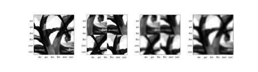
Image example

% Again, the image center is not in (1,1).  It is in the center.
tmp = load('trees');
cmap = gray(128);
imgC = cmap(tmp.X);
imgC = imgC(1:theDim,1:theDim);
ieNewGraphWin([],'wide');
subplot(1,4,1); colormap(gray(64)); imagesc(imgC); axis image

% Before we transform the image, we want to place its center in the (1,1)
% position.  This produces a weird looking beast, but it is what fft2 wants
% as its input.
imgForFT = ifftshift(imgC);
subplot(1,4,2); imagesc(imgForFT); axis image

% Then we compute the transform
imgFT = fft2(imgForFT);

% If we hadn't done the ifftshift, we'd still get the same absolute value
% of the FT to numerical precision. One thing that makes keeiping the all
% the fftshift stuff straight difficult is that for various special cases
% the ifftshift doesn't matter.  The code below demonstrates that here the
% difference is only in the phase.
imgFTNoShift = fft2(imgC);
if (max(abs(imgFT(:)) - abs(imgFTNoShift(:))) > 1e-10)
    fprintf('Surprising difference in FFT modulus with insertion of ifftshift\n');
else
    fprintf('FFT modulus behaves as expected with insertion of ifftshift\n');
end
if (max(angle(imgFT(:)) - angle(imgFTNoShift(:))) > 1e-10)
    fprintf('Expected difference in FFT phase with insertion of ifftshift\n');
else
    fprintf('FFT phase unexpectedly preserved with insertion of ifftshift\n');
end

% We are ready to multiply the transformed image and the OTF
imgFTgFT = imgFT .* gFT;

% We can return the transform to the space domain.
imgConvG = ifft2(imgFTgFT);

% When we do, the image center is still in the (1,1) position.
subplot(1,4,3); colormap(gray(64)); imagesc(imgConvG); axis image

% We want the center in the center.  So we apply fftshift.
imgConvGCentered = fftshift(imgConvG);
subplot(1,4,4); imagesc(imgConvGCentered); axis image

FFT modulus behaves as expected with insertion of ifftshift
Expected difference in FFT phase with insertion of ifftshift

Contents