t_codeTikhonovRidge

Explain Tikhonov regularizer (ridge, regression)

Implementation is based on wikipedia and other stuff we know.

https://en.wikipedia.org/wiki/Ridge_regression#Tikhonov_regularization

This explains the calculation when we solve b = Ax, subject to different constraints ('min norm',lambda) or ('smooth',lambda)

   x = ieTikhonov(A,b,varargin);

Contents

Consider an ordinary linear equation

b = Ax

% Here is an example.  Underconstrained equation
A = rand(20,10);   % 20 x 10  matrix
b = rand(20,1);    % Predict 20 numbers
x = A\b;           % Only 10 free parameters

bhat = A*x;      % The predicted value of b

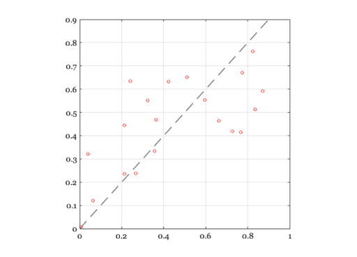
This is how much we miss with ordinary least squares

ieNewGraphWin;
plot(b(:),bhat(:),'o');
identityLine;
axis square;
norm(b - A*x )

ans =

    0.9339

This is what x looks like

The Tikhonov regression

Find a shorter solution, x. How much do we care? lambda

x = argmin b-Ax^2 + lambda*|x|^2

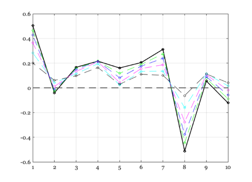
%  The closed form Tikhonov solution.  Notice that the curves shrink
%  towards the y = 0 line, making the solution vector length smaller.  The
%  error gets larger as lambda gets larger.
ieNewGraphWin;
plot(x,'-ko','LineWidth',2);
hold on;
for lambda = logspace(-1,0.5,5)
    xR = inv(A'*A + lambda*eye(size(A,2))) * A' * b;
    plot(xR,'--o');
    fprintf('Err %.2f Mag %.2f\n',norm(b - A*xR),norm(xR));
end
xaxisLine;

Err 0.94 Mag 0.79
Err 0.95 Mag 0.71
Err 0.98 Mag 0.59
Err 1.04 Mag 0.46
Err 1.12 Mag 0.35

Smoother solutions

% We can use an alternative regularizer to impose a different
% constraint on the solution, x. We might like a smoothness
% constraint, say to mimize the magnitude of the 2nd derivative.
%
% x = argmin |b - Ax|^2 + lambda*|D2*x|^2

% In this case, D is the first derivative operator expressed as a matrix, sometimes
% called the difference operator.

% There is a direct solution for this case

D2 = diff(eye(size(A,2)), 2);  % Second-order finite difference matrix

The sum of the terms is how chatGPT put it.

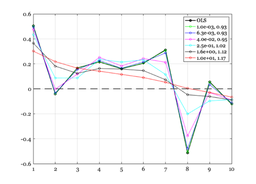
lgn = cell(1,7);
% We want it smooth, but we do not care if it has a smaller norm.  We set
% lambda to 1 (ignore it).
ieNewGraphWin;
plot(x,'-ko','LineWidth',2);
ii = 1; lgn{1} = 'OLS';
for lambda2 = logspace(-3,1,6)
    xD = inv(A'*A + eye(size(A,2)) + lambda2*(D2'*D2)) * A' * b;
    hold on;
    p = plot(xD,'-o');
    % lgn{ii} = sprintf('%.1f',norm(b - A*xD));
    ii = ii+1; lgn{ii} = sprintf('%.1e, %.2f',lambda2, norm(b-A*xD));
    %    norm(b - A*xD)
end
xaxisLine;
legend(lgn);

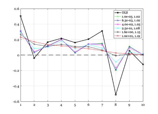
The wikipedia formula

% We want it smooth, but we do not care if it has a smaller norm.
ieNewGraphWin;
plot(x,'-ko','LineWidth',2);
ii = 1; lgn{1} = 'OLS';
for lambda2 = logspace(-3,1,6)
    xD = inv(A'*A + lambda2*(D2'*D2)) * (A' * b); %#ok<*MINV>
    hold on;
    p = plot(xD,'-o');
    % lgn{ii} = sprintf('%.1f',norm(b - A*xD));
    ii = ii+1; lgn{ii} = sprintf('%.1e, %.2f',lambda2, norm(b-A*xD));
    %    norm(b - A*xD)
end
xaxisLine;
legend(lgn);

% Computational efficiency trick from Haomiao.
%
%  By SVD, we can avoid the matrix inversion and estimate the
%  coefficients as
%    [U, S, V'] = svd(A);
%    s = diag(S);
%    x = V * diag(s./(s.^2 + lambda))*U'*b

%}

Published with MATLAB® R2024a