CIE error metric plots

The CIELAB color space and its associated distance ( $\Delta E$ ) are widely used to specify color discrimination. Although there are now modern extensions (e.g., CIECAM02), CIELAB remains in wide use.

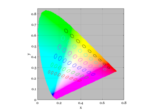
This script plots the iso $\Delta E$ contours around different coordinates in XYZ space. It also shows the ellipses for equal L*=50 level on the chromaticity diagram.

From these plots, we see the non-uniformity of color discrimination in CIE XYZ space, and the need for a nonlinear metric (CIELAB).

See also: ieLAB2XYZ, ieCirclePoints, ieDrawShape, daylight Copyright Imageval 2012

Choose a white point for the calculation
Choose the Lab centers
XYZ plot
Chromaticity plot (x,y)
Make a sphere for Lab
Add the sphere to the centers and plot the XYZ values

ieInit

Choose a white point for the calculation

% Blackbody, 5000K
wave = 400:10:700;
[~, whiteXYZ] = daylight(wave,5000);

% Make circle of points in (a,b) coordinates
nSamples = 20;
radSpacing = 2*pi/nSamples;  % Radial spacing
[a,b] = ieCirclePoints(radSpacing);
% vcNewGraphWin; plot(a,b,'o'); axis equal

% Put them at the proper radius
dE = 5;
dAB = dE*[a(:),b(:)];
dLab = cat(2,zeros(size(dAB,1),1),dAB);
% vcNewGraphWin; plot3(dLab(:,1),dLab(:,2),dLab(:,3),'o');

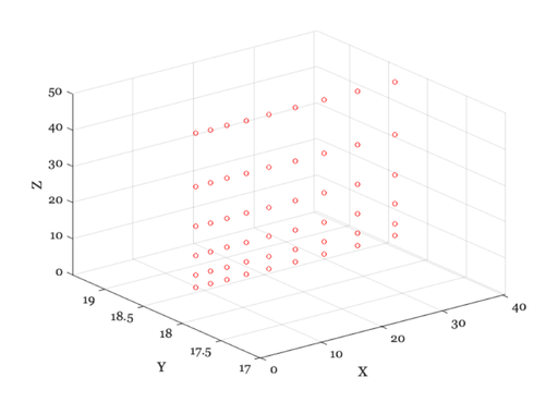
Choose the Lab centers

% Alternate values you could try
%   amn = -80;
%   amx =  80;
%   bmn = -90;
%   bmx = 90;
%   L = 70;

% Minimum and maximum ranges for a,b coordinates
amn = -70;
amx =  90;
bmn = -50;
bmx = 50;
L = 50;

[a,b] = meshgrid(amn:20:amx,bmn:20:bmx);
AB    = [a(:), b(:)];
lab0 = cat(2,L*ones(size(AB,1),1),AB);

% Convert the LAB points into XYZ points
XYZ0 = ieLAB2XYZ(lab0,whiteXYZ);

% Plot the XYZ points
vcNewGraphWin; plot3(XYZ0(:,1),XYZ0(:,2),XYZ0(:,3),'o');
xlabel('X'); ylabel('Y'); zlabel('Z'); grid on

% lab0  = [100 0 0; 50 -20 0; 50 20 0; 20 0 -30 ; 100 0 30];
nCenters = size(lab0,1);
nSamp    = size(dLab,1);

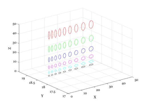
XYZ plot

vcNewGraphWin;
for ii = 1:nCenters
    lab  = dLab + repmat(lab0(ii,:),[nSamp,1]);
    xyz = ieLAB2XYZ(lab,whiteXYZ);
    % Just the points.
    plot3(xyz(:,1),xyz(:,2),xyz(:,3),'-'); grid on
    hold on
end
xlabel('X'); ylabel('Y'); zlabel('Z');

Chromaticity plot (x,y)

chromaticityPlot; hold on
for ii = 1:nCenters
    lab  = dLab + repmat(lab0(ii,:),[nSamp,1]);
    xy = chromaticity(ieLAB2XYZ(lab,whiteXYZ));
    % Just the points.
    plot(xy(:,1),xy(:,2),'-'); grid on
    hold on
end
xlabel('x'); ylabel('y');

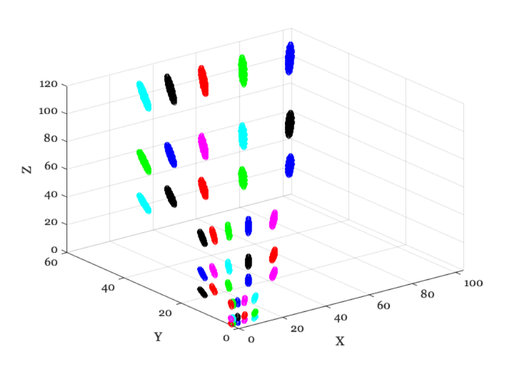
Make a sphere for Lab

N = 15;
[L, a, b] = sphere(N);
% vcNewGraphWin;
% surf(L,a,b); colormap(hot(64))

% These are the sphere points at 5 dE
dLab    = 2*[L(:),a(:),b(:)];
nSamp = size(dLab,1);

% Now make the centers, widely spaced for this 3D case
amn = -70;
amx =  90;
bmn = -50;
bmx = 50;
Lmn = 20;
Lmx = 80;

[L,a,b] = meshgrid(Lmn:30:Lmx,amn:40:amx,bmn:40:bmx);
lab0    = [L(:), a(:), b(:)];
nCenters = size(lab0,1);

Add the sphere to the centers and plot the XYZ values

vcNewGraphWin;
for ii = 1:nCenters
    lab  = dLab + repmat(lab0(ii,:),[nSamp,1]);
    XYZ = ieLAB2XYZ(lab,whiteXYZ);

    % Just the points.
    plot3(XYZ(:,1),XYZ(:,2),XYZ(:,3),'o'); grid on
    hold on
end
xlabel('X'); ylabel('Y'); zlabel('Z')