The slanted Bar and ISO 12233 metric

The ISO 12233 standard defines a modulation transfer function for assessing system acuity.

This script also illustrates how to # define a scene # create an optical image from the scene # define a monochrome sensor # evaluate the sensor MTF

We measure the system MTF properties using a simple slanted bar target along with the ISO 12233 standard methods.

This script is an example of a complicated (but useful) calculation. We suggest that you begin programming scripts using other, simpler routines. We include this script because it shows many features of the scripting language and the ability to interact with the GUI from scripts.

See also: ieISO12233, ieISO12233v1, s_pixelSizeMTF, ISOFindSlantedBar, ieDrawShape, ipCompute

First, create a slanted bar image. Make the slope some uneven value
Create an optical image with some default optics.
Create a default monochrome image sensor array
Run the computation for the monochrome sensor
Should be the same, but from the ie routine
Updated with with sfrmat4
Now for a monochrome sensor
You can also get the MTF and LSF data from figure
Plot the MTF
END

ieInit

First, create a slanted bar image. Make the slope some uneven value

sz = 512;    %Row and col samples
slope = 7/3;
meanL = 100; % cd/m2
viewD = 1;   % Viewing distance (m)
fov   = 5;   % Horizontal field of view  (deg)

scene = sceneCreate('slantedBar',sz,slope);

% Now we will set the parameters of these various objects.
% First, let's set the scene field of view.
scene = sceneAdjustLuminance(scene,meanL);    % Candelas/m2
scene = sceneSet(scene,'distance',viewD);       % meters
scene = sceneSet(scene,'fov',fov);            % Field of view in degrees

Create an optical image with some default optics.

oi = oiCreate;

fNumber = 2;
optics = oiGet(oi,'optics');
optics = opticsSet(optics,'fnumber',fNumber);
oi = oiSet(oi,'optics',optics');

% Now, compute the optical image from this scene and the current optical
% image properties
oi = oiCompute(oi,scene);

Create a default monochrome image sensor array

sensorM = sensorCreate('monochrome');   % Monocrhome sensor
sensorC = sensorCreate;                 % RGB sensor

sensorM = sensorSet(sensorM,'autoExposure',1);
sensorC = sensorSet(sensorC,'autoExposure',1);

% We are now ready to set sensor and pixel parameters to produce a variety
% of captured images. Set the rendering properties for the monochrome
% imager. The default does not color convert or color balance, so it is
% appropriate.
ip = ipCreate;

% To see the scene, optical image, sensor or virtual camera image in the
% GUI, use these commands
%    vcReplaceObject(scene); sceneWindow;
%    vcReplaceObject(oi); oiWindow;
%    vcReplaceObject(sensor); sensorWindow;
%    vcReplaceObject(vci); ipWindow;

% To determine the masterRect size, run this code and use the
% measured values of masterRect.
%
%    sensor = sensorCompute(sensor,oi);
%    vcReplaceObject(sensor);
%    vci = ipCompute(vci,sensor);
%    vcReplaceObject(vci); ipWindow;
%    [roiLocs,masterRect] = vcROISelect(vci);
%
%    masterRect = [ 27    13    35    53];   % October 2, 2010

Run the computation for the monochrome sensor

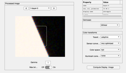
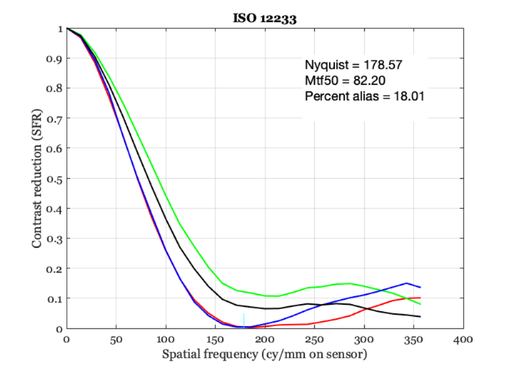
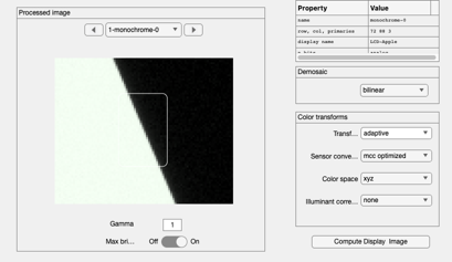
sensor = sensorCompute(sensorC,oi);
vcReplaceObject(sensor);
ip = ipCompute(ip,sensor);
vcReplaceObject(ip); ipWindow;

% Find a good rectangle
masterRect = ISOFindSlantedBar(ip);
h = ieDrawShape(ip,'rectangle',masterRect);

barImage = vcGetROIData(ip,masterRect,'results');
c = masterRect(3)+1;
r = masterRect(4)+1;
barImage = reshape(barImage,r,c,3);
% vcNewGraphWin; imagesc(barImage(:,:,1)); axis image; colormap(gray(64));

% Run the ISO 12233 code.  The results are stored in the window.
pixel = sensorGet(sensor,'pixel');
dx = pixelGet(pixel,'width','mm');
ISO12233(barImage, dx)

No black border detected

ans = 

  struct with fields:

                  freq: [26×1 double]
                   mtf: [26×4 double]
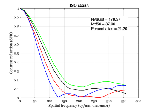
              nyquistf: 178.5714
                   lsf: [100×1 double]
                  lsfx: [-0.0693 -0.0679 -0.0665 -0.0651 … ] (1×100 double)
                 mtf50: 87
    aliasingPercentage: 21.1996

Should be the same, but from the ie routine

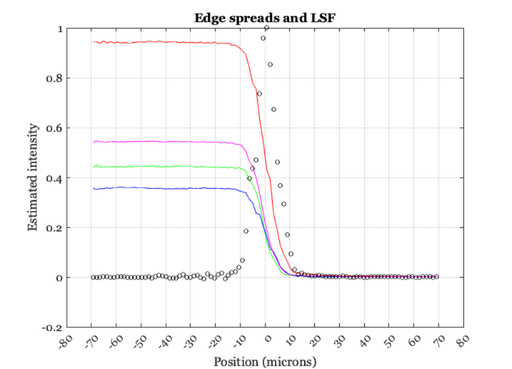
% From the 2001 functions
mtfData = ieISO12233(ip,sensor);
ieNewGraphWin;
plot(mtfData.lsfx*1e3,mtfData.esf); grid on;
xlabel('Position (microns)'); ylabel('Estimated intensity')
title('Edge spreads and LSF');
set(gca,'xtick',-80:10:80)
hold on;
plot(mtfData.lsfx*1e3,mtfData.lsf,'ko');

No black border detected

Updated with with sfrmat4

mtfData = ieISO12233(ip,sensor);
ieNewGraphWin;
plot(mtfData.lsfx*1e3,mtfData.esf); grid on;
xlabel('Position (microns)'); ylabel('Estimated intensity')
title('Edge spreads and LSF');
set(gca,'xtick',-80:10:80)
hold on;
plot(mtfData.lsfx*1e3,mtfData.lsf,'ko');

No black border detected

Now for a monochrome sensor

sensor = sensorCompute(sensorM,oi);
vcReplaceObject(sensor);

ip = ipCompute(ip,sensor);
vcReplaceObject(ip); ipWindow;
h = ieDrawShape(ip,'rectangle',masterRect);
% To get rid of the bar, use:  delete(h)
% or just refresh

barImage = vcGetROIData(ip,masterRect,'results');
c = masterRect(3)+1;
r = masterRect(4)+1;
barImage = reshape(barImage,r,c,3);
% vcNewGraphWin; imagesc(barImage(:,:,1)); axis image; colormap(gray(64));

% Run the ISO 12233 code.  The results are stored in the window.
dx = sensorGet(sensor,'pixel width','mm');

% Run the code, and plot
mtfData = ISO12233(barImage, dx, [], 'all');

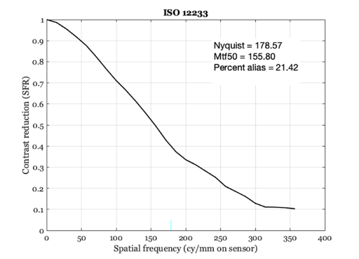
You can also get the MTF and LSF data from figure

% The mtfData variable contains all the information plotted in this figure.
% We graph the results again just to illustrate what is in the data
% structure.
%
%  mtfData = get(gcf,'userdata');
%

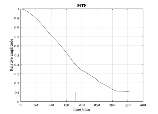
Plot the MTF

ieNewGraphWin;
h = plot(mtfData.freq,mtfData.mtf,'-k');
hold on
nfreq = mtfData.nyquistf;
l = line([nfreq ,nfreq],[0.1,0],'color','k');
% text((nfreq-10),0.12,newText,'color','k');
xlabel('lines/mm');
ylabel('Relative amplitude');
title('MTF');
hold off; grid on

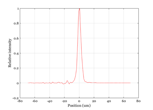
ieNewGraphWin;
plot(mtfData.lsfx*1000, mtfData.lsf);
xlabel('Position (um)'); ylabel('Relative intensity');
grid on