s_opticsPSF2OTF

Start with an image (e.g., from Flare 7K) that defines a PSF. Then define the pixel size. Convert the image into a properly labeled OTF struct that can be attached to a shift-invariant OI.

See also opticsPSF2OTF

Contents

We first just get the PSF into the OTF format with the proper fftshift

fname = fullfile(isetRootPath,'data','optics','flare','flare1.png');
OTF = opticsPSF2OTF(fname,1.2e-6,400:10:700);

Put the OTF struct into OI.optics

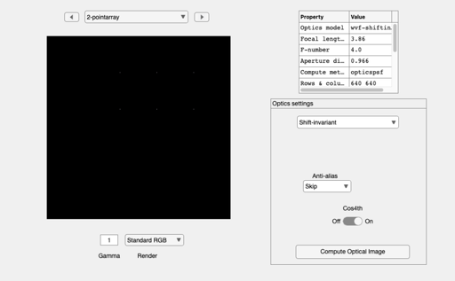
scene = sceneCreate('point array',512, 128);
scene = sceneSet(scene,'hfov',40);

oi = oiCreate('shift invariant');
oi = oiSet(oi,'optics otf struct',OTF);
oi = oiCompute(oi,scene);

oiWindow(oi);

END

%{
% Zhenyi/Brian developed the code here and moved it into the function,
% opticsPSF2OTF
%
img = imread(fname);
psf = img(:,:,2);   % Use the green channel
% ieNewGraphWin; imagesc(psf); colormap(gray)

psf = double(psf);
psf = psf/sum(psf(:));

[row,col] = size(psf);

% We need to expand this over wavelengths
% otf = ifft2(psf);
% otf = psf2otf(psf); % from matlab builtin
% psf_shift = circshift(psf, -floor(size(psf)/2)); % from matlab builtin
psf_shifted = fftshift(psf);
otf = fft2(psf_shifted);
%%
% The DC is NOT in the center.  So to see the whole pattern we
% fftshift it into the center
% ieNewGraphWin; imagesc(fftshift(abs(otf)));
% ieNewGraphWin; mesh(fftshift(abs(otf)));

%% Then we figure out the cycles per millimeter

hFOV     = 40;       % Horizontal field of view in degrees
pixSize  = 1.2e-6;   % Standard might be 1.2 microns
imgSizeM = pixSize*col;   % Image size in meters
imgSizeMM = imgSizeM*1e3; % Image size in millimeters

% OTF frequencies are stored in cycles per degree
fx = (-(col/2):( (col/2)-1) ) * (1/imgSizeMM);
fy = (-(row/2):( (row/2)-1) ) * (1/imgSizeMM);

%% Again to visualize now with frequencies labeled

% ieNewGraphWin; imagesc(fx,fy,fftshift(abs(otf)));
% ieNewGraphWin; mesh(fx,fy,fftshift(abs(otf)));
%}

Published with MATLAB® R2024a