Contents

% Adaptive optics data for the human point spread function
%
% Description:
%    Using adaptive optics, a group led by Thibos collected many different
%    wavefronts in the human eye for a range of pupil sizes.  The data are
%    summarized using a simple statistical model of the Zernicke polynomial
%    coefficients. The data were published in
%
%    "Retinal Image Quality for Virtual Eyes Generated by a Statistical
%    Model of Ocular Wavefront Aberrations" published in Ophthalmological
%    and Physiological Optics (2009). Thibos, Ophthalmic & Physiological
%    Optics. http://onlinelibrary.wiley.com/doi/10.1111/...
%    j.1475-1313.2009.00662.x/full
%
%    The data and a sample program are online at the bottom of the online
%    article in Supporting Information.
%
%    We retrieved the data and implemented a version of the calculations in
%    the Wavefront toolbox. This script calculates the PSF for example
%    subjects.
%
% See Also:
%    wvfLoadThibosVirtualEyes
%  http://onlinelibrary.wiley.com/doi/10.1111/j.1475-1313.2009.00662.x/full
%

% History:
%    xx/xx/12       Copyright Wavefront Toolbox Team, 2012
%    12/21/17  dhb  Comments
%    09/25/18  jnm  Formatting

Initialize ISET

Set the largest size in microns for plotting Set the pupil diameter in millimeters

ieInit;

maxUM = 30;
measPupilMM = 4.5;  % This selects which Thibos data set to load
calcPupilMM = 3.0;  % Calculate for this pupil size

Load the statistical wavefront properties

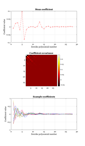
The Zernike coefficients describing the wavefront aberrations are each distributed as a Gaussian. There is some covariance between these coefficients. The covariance is summarized in the variable S. The mean values across a large sample of eyes measured by Thibos and gang are in the variable sample_mean.

[sample_mean, S] = wvfLoadThibosVirtualEyes(measPupilMM);

Plot the means and covariance (not)

ieNewGraphWin([], 'tall');

subplot(3, 1, 1)
plot(sample_mean, '--o');
grid on
xlabel('Zernike polynomial number')
ylabel('Coefficient value')
title('Mean coefficient');

subplot(3, 1, 2)
imagesc(S);
axis image,
colormap(hot);
colorbar
title('Coefficient covariance')

% Calculate sample eyes using the multivariate normal distribution Each
% column of Zcoeffs is an example person. Each row of R is a vector of
% Zernike coeffs
N = 10;
Zcoeffs = ieMvnrnd(sample_mean, S, N)';

% Plot the random examples of coefficients
subplot(3, 1, 3)
plot(Zcoeffs);
grid on
xlabel('Zernike polynomial number')
ylabel('Coefficient value')
title('Example coefficients')

Examine a single PSF for the subject at the sample mean

Allocate space and fill in the lower order Zernicke coefficients

z = zeros(65, 1);
z(1:13) = sample_mean(1:13);

Create the example subject

Initialize

thisGuy = wvfCreate;

% Set Zernicke, and add data
thisGuy = wvfSet(thisGuy, 'zcoeffs', z);
thisGuy = wvfSet(thisGuy, 'measured pupil', measPupilMM);

% Calculation
thisGuy = wvfSet(thisGuy, 'calculated pupil', calcPupilMM);
thisGuy = wvfSet(thisGuy, 'measured wavelength', 550);

% Set to column vector
thisGuy = wvfSet(thisGuy, 'calc wave', [450:100:650]');
thisGuy = wvfCompute(thisGuy);

Plot the PSFs of the sample mean subject for several wavelengths

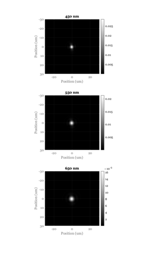
These illustrate the strong axial chromatic aberration.

wave = wvfGet(thisGuy, 'calc wave');
nWave = wvfGet(thisGuy, 'calc nwave');
ieNewGraphWin([], 'tall');
for ii = 1:nWave
    subplot(nWave, 1, ii)
    wvfPlot(thisGuy, 'image psf', 'unit','um', 'wave', wave(ii), 'plot range',maxUM, ...
        'window', false);
    title(sprintf('%d nm', wave(ii)));
    colorbar
end
colormap(gray(256));

Calculate the PSFs from the coeffcients

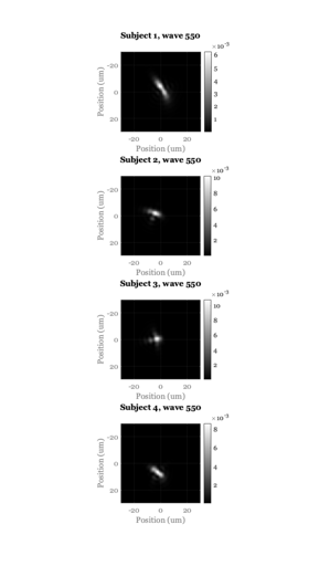
Here we illustrate the variance between different subjects.

% Choose example subjects
whichSubjects = 1:3:N;
nSubjects = length(whichSubjects);
z = zeros(65, 1);  % Allocate space for the Zernicke coefficients

Create the example subject

Initialize and set data

thisGuy = wvfCreate;
thisGuy = wvfSet(thisGuy, 'measured pupil', measPupilMM);

% What we calculate
thisGuy = wvfSet(thisGuy, 'calculated pupil', calcPupilMM);

ieNewGraphWin([], 'tall');
thisWave = wave(1);
for ii = 1:nSubjects
    % Choose different coefficients and compute for each subject
    z(1:13) = Zcoeffs(1:13, whichSubjects(ii));
    thisGuy = wvfSet(thisGuy, 'zcoeffs', z);  % Zernike

    thisGuy = wvfSet(thisGuy, 'calc wave', thisWave);
    thisGuy = wvfCompute(thisGuy);

    subplot(nSubjects, 1, ii)
    wvfPlot(thisGuy, 'image psf', 'unit','um', 'wave', thisWave, 'plot range', maxUM, ...
        'window', false);
    title(sprintf('Subject %i, wave %i\n', ii, thisWave));
    colorbar;
end
colormap(gray(256));

ieNewGraphWin([], 'tall');
thisWave = wave(2);
for ii = 1:nSubjects
    % Choose different coefficients and compute for each subject
    z(1:13) = Zcoeffs(1:13, whichSubjects(ii));
    thisGuy = wvfSet(thisGuy, 'zcoeffs', z);  % Zernike

    thisGuy = wvfSet(thisGuy, 'calc wave', thisWave);
    thisGuy = wvfCompute(thisGuy);

    subplot(nSubjects, 1, ii)
    wvfPlot(thisGuy, 'image psf', 'unit','um', 'wave', thisWave, 'plot range', maxUM, ...
        'window', false);
    title(sprintf('Subject %i, wave %i\n', ii, thisWave));
    colorbar;
end
colormap(gray(256));

END

Published with MATLAB® R2024a