Plot the wavefront aberrations of Zernike polynomial coefficients

https://en.wikipedia.org/wiki/Zernike_polynomials

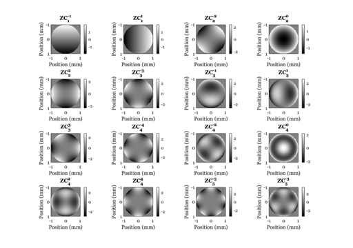
Compare the computed wavefronts by our wvf with the Zernike functions based on (zernfun). This is downloaded from the web.

They are, of course, the same. Except! there is a flipud somewhere and there is a scale factor (sqrt(pi) ~ 1.77) in the zernfun that we undo.

See also wvf2oi, wvfCreate, wvfCompute

Contents

ieInit;

Create wavefront object and convert it to an optical image object

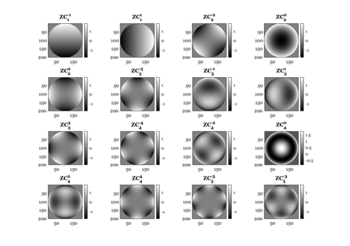
uData = cell(16,1);

ieNewGraphWin([],'upper left big');
for ii=1:16
    subplot(4,4,ii);
    wvf = wvfCreate;   % Creates just 0
    wvf = wvfSet(wvf,'npixels',801);             % Higher resolution
    wvf = wvfSet(wvf,'measured pupil size',2);   % This is diameter
    wvf = wvfSet(wvf,'calc pupil size',2);       % This is diameter
    wvf = wvfSet(wvf,'zcoeff',1,ii);
    wvf = wvfCompute(wvf);
    [n,m] = wvfOSAIndexToZernikeNM(ii);
    uData{ii} = wvfPlot(wvf,'image wavefront aberrations','unit','mm','wave',550,'plot range',1,'window',false);
    colormap("gray"); title(sprintf('ZC_{%d}^{%d}',n,m));
end

Our values are flipped updown compared to these

ieNewGraphWin([],'upper left big');

% Over the unit radius disk.  Diameter is 2.
x = -1:0.01:1;
[X,Y] = meshgrid(x,x);
[theta,r] = cart2pol(X,Y);
idx = r<=1;

% Makes the outside region 0 (gray)
z = zeros(size(X));

% zernfun multiplies by 1/sqrt(pi) relative to the OSA standard.  We
% compensate here.  Maybe we should make our own version of zernfun
% that does not require this adjustment?
for ii=1:16
    subplot(4,4,ii);
    [n,m] = wvfOSAIndexToZernikeNM(ii);
    z(idx) = sqrt(pi)*zernfun(n,m,r(idx),theta(idx));
    imagesc(flipud(z)); axis square;
    colormap('gray'); colorbar;
    title(sprintf('ZC_{%d}^{%d}',n,m));
end

Published with MATLAB® R2024a