Contents
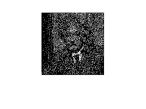
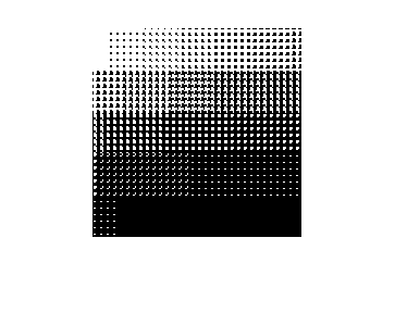
%t_Halftone - Printing tutorial
%
%PURPOSE:  Image halftoning for binary, black/white, printers
%AUTHOR:   R. Koehler, X. Zhang, B. Wandell
%DATE:     02.25.97
%CONCEPTS:
%
% This tutorial illustrates how to use halftoning to achieve the
% visual illusion of gray-levels in a binary display system.
% You will learn about two approaches:  thresholding approaches
% using dither patterns and the computational method called error
% diffusion.
%
% Matlab 7:  Checked 01.08.06
% Matlab 5:  Checked 01.06.98
%
%%%%%%%%%%%%%%%%%%%%%%%%%%%%%%%%%%%%%%%%%%%%%%%%%%%%%%%%%%%%%%%%%

% Most printers place a binary mark at each spot on the page:
% that is, they either place a dot at position or not. Hence,
% unlike monitors, printers do not display a range of intensity
% levels.

% To create the illusion of intensity variation, printers fool
% the eye by trading area for intensity.  One way to do this is
% to divide the image into a number of small areas (halftone
% cells) and print more or less dots in this area according to a
% rule that is governed by the local image intensity.  This
% halftoning process substitutes a number of dots for a variation
% in gray level (or color).

% The algorithm for simple halftoning is to define a small
% pattern, defined over the halftone cell, that spans a small
% number of printable dots.  The values within this halftone cell
% define a set of thresholds.  The binary decision of whether to
% print or not at each addressable print location is governed by
% how the image intensity compares to the entry in the halftone
% cell.  Halftone algorithms are often named by the principle
% that underlies the pattern within the halftone cell.

% Let's begin with a simple halftone algorithm called "cluster dot."
% This algorithm uses a halftone cell in which the printed area
% has the shape of a larger and larger dot.  As the image region
% within the halftone cell becomes darker and darker, the size of
% the dot grows larger.  Here is an example of a 4x4 halftone
% cell that illustrates the idea.

halfToneCell_4 = ...
    [15 5 12 14
    10 3 2 8
    7 1 4 11
    13 9 6 16];

% Suppose we have a 4x4 image region that has a hight density,
% say 12.
im = 12*ones(4,4);

% To print this section of the image, we compare the density in
% the image with the thresholds in the halftone cell,
cmp = halfToneCell_4 < im

%  The locations set to one are printed with a black dot, and the
% locations with 0 are unprinted (white).  Because of Matlab's
% ordering, we will add 1 to cmp and build the binary color map
% as
bMap = [1 1 1; 0 0 0]

figure;
colormap(bMap); image( cmp + 1 );

% For this high density, we print most of the halftone cell as
% black.  Now, let's see how the halftone cell would print at a
% set of increasing densities:

cnt = 1;
for density = 1:16
    im = ones(4,4)*density;
    cmp = (halfToneCell_4 < im);
    subplot(4,4,cnt)
    image(cmp + 1);
    cnt = cnt + 1;
end

% As the mean image density varies from low (light) to high
% (dark) the region corresponding to the halftone cell is printed
% as an increasingly large black dot.

% Now we can apply the halftone cell to an entire test image.
% We start with a simple test image containingeight gray strips
% that vary from black to white.

grayStrips = 8;
bw_range = [0, 1];
sweep_size = 128;

%
[x,y] = meshgrid(0:sweep_size-1, 0:sweep_size-1);
y = fix(y * grayStrips / sweep_size) / grayStrips;
x = x / (sweep_size * grayStrips);
sweep_8 = ones(sweep_size, sweep_size) - (x + y);

% This ramp pattern has many gray levels arranged in 8 strips.
% The density increases from left to right.
figure;
imshow(sweep_8);

% The values in sweep_8 are frame buffer values that are
% nonlinearly related to intensity.  The halftoning principle
% depends on LINEAR SPATIAL AVERAGING of the dots.  Hence, to
% make the proper decisions about the halftoning, we have to take
% into account the true intensity associated with each level.
% Hence, before halftoning we need to convert the frame buffer
% values to linear gray scale values (gamma correction--review
% the ColorMatching tutorial for why and how to perform gamma
% correction). We use a gamma value = 2.

monitorGamma = 2;
sweep_8_linear = sweep_8 .^ monitorGamma;
HTsweep_4 = HalfToneImage(halfToneCell_4, sweep_8_linear);
imshow(HTsweep_4);

% Were we doing this on a printer, rather than a display, we
% would have to know the relationship between the image density
% and the displayed intensity, and also, we would need to know
% the relationship between the image dot size in the cluster dot
% and the reflected intensity.

% The image halftone is created in the routine
% HalfToneImage. (Use type HalfToneImage to see the full
% routine).  The process simply applies the HalfToneCell
% comparison again and again across the image.  The light image
% regions contain no black dot or a small black dot.  The dark
% image regions contain large black dots or a complete black dot.

type HalfToneImage.m

% The halftone does a worse job tracking the gray levels if the
% halftone cell is smaller.

halfToneCell_2 = [ 4 3; 2 1];
HTsweep_2 = HalfToneImage(halfToneCell_2, sweep_8_linear);
imshow(HTsweep_2);

% We can also scale up these two images to see how the halftones are formed.
%
scale_sweep_2 = kron(HTsweep_2, ones(3,3));
imshow(scale_sweep_2);

scale_sweep_4 = kron(HTsweep_4, ones(3,3));
imshow(scale_sweep_4);

%%%%%%%%%%%%%%%%%%%%%%%%%%%%%%%%%%%%%%%%%%%%
%
% Bayer dithering
%
%%%%%%%%% %%%%%%%%% %%%%%%%%% %%%%%%%%% %%%%%%%%%

% In the supplemental reading, Bayer describes a halftone cell
% for Figure 2: "imitation halftone pattern."  We enter it as:

halfToneCell_B2 = ...
    [7 6 5 16 17 18 19 20
    8 1 4 15 28 29 30 21
    9 2 3 14 27 32 31 22
    10 11 12 13 26 25 24 23
    17 18 19 20 7 6 5 16
    28 29 30 21 8 1 4 15
    27 32 31 22 9 2 3 14
    26 25 24 23 10 11 12 13];

colormap(bMap)
cnt = 1;
for density = 1:32
    im = ones(8,8)*density;
    cmp = (halfToneCell_B2 < im);
    subplot(6,6,cnt)
    image(cmp + 1);
    cnt = cnt + 1;
end

% This pattern is much like the simple cluster dot, except it
% introduces a smaller pair of dots oriented at 45 deg to the
% image. Now apply it to the sweep pattern:
clf
HTsweep_B2 = HalfToneImage(halfToneCell_B2, sweep_8_linear);
imshow(HTsweep_B2);

% Bayer also describes a halftone cell for Figure 4 that
% considered to be much better (he called it an "optimum dot
% pattern").  This pattern is built so that the dots are
% dispersed in a random array.

halfToneCell_B4 = ...
    [1 17 5 21 2 18 6 22
    25 9 29 13 26 10 30 14
    7 23 3 19 8 24 4 20
    31 15 27 11 32 16 28 12
    2 18 6 22 1 17 5 21
    26 10 30 14 25 9 29 13
    8 24 4 20 7 23 3 19
    32 16 28 12 31 15 27 11];

figure;
colormap(bMap)
cnt = 1;
for density = 1:32
    im = ones(8,8)*density;
    cmp = (halfToneCell_B4 < im);
    subplot(6,6,cnt)
    image(cmp + 1);
    cnt = cnt + 1;
end

clf
HTsweep_B4 = HalfToneImage(halfToneCell_B4, sweep_8_linear);
imshow(HTsweep_B4);

% if you want to close the image windows, do this
close all;

% These halftones can also be applied to a real image.

D = load('jpegFiles/einstein.mat'); img = D.X;
img = img / 256;
imshow(img);

% gamma correction
img_linear = img .^ monitorGamma;

HTimg_B4 = HalfToneImage(halfToneCell_B4, img_linear);
imshow(HTimg_B4);

% If you enlarge this image you should see that the halftone
% cells are not the same as the basic patterns we saw.  This is
% because the halftone dot is formed by the space-varying image
% not simple constant patterns. The image changes density rapidly
% over sapce and the dots reflect the correct image density.

scale_img_B4 = kron(HTimg_B4, ones(3,3));
imshow(scale_img_B4);

% You can see this easily by changing the original sweep to
% a different number of strips, say 5.  Thus the halftone
% cells will not line up on the strip boundaries.

grayStrips = 5;
[x,y] = meshgrid(0:sweep_size-1, 0:sweep_size-1);
y = fix(y * grayStrips / sweep_size) / grayStrips;
x = x/(sweep_size * grayStrips);
sweep_5 = ones(sweep_size, sweep_size) - (x + y);
imshow(sweep_5);

% gamma correction
%
sweep_5_linear = sweep_5 .^ monitorGamma;

HTsweep_5_4 = HalfToneImage(halfToneCell_4, sweep_5_linear);
imshow(HTsweep_5_4);

scale_sweep_5_4 = kron(HTsweep_5_4, ones(3,3));
imshow(scale_sweep_5_4);
cmp =

  4×4 logical array

   0   1   0   0
   1   1   1   1
   1   1   1   1
   0   1   1   0


bMap =

     1     1     1
     0     0     0


function htimage = HalfToneImage(cell, im)
%
%            htimage = HalfToneImage(cell, im)
%
% AUTHOR:  Koehler, Zhang, Wandell
% DATE:    02.25.97
% PURPOSE:
%
% This function takes in a halftone cell and an image as
% arguments.
%    cell: An array of threshold levels.  If these exceed 1, then
%          the cell is scaled to evenly spaced values between 0 and 1.
%          If the numbers all fall between 0 and 1, then they are
%          left as they are.
%    im:   The image gray levels, values between 0 and 1.
%
% htimage: The returned halftone image.  Its values are set to 0
% (white) or 1 (black).  The binary color map is [ 1 1 1; 0 0 0];

% DEBUGGING:
% im = (rand(32,32)).^2;
% cell = [ 1 2 ; 3 4];

imSize = size(im);
cellSize = size(cell);

% The cell thresholds should fall at the midpoints of the
%
if max(cell) > 1
    low = (1/max(cell(:)))*0.5; high = 1 - low;
    halfToneCell = ieScale(cell,low,high);
else
    halfToneCell = cell;
end

% Determine number of halftone cells needed to cover the image
%
rc = imSize ./ cellSize;
r = ceil(rc(1));
c = ceil(rc(2));

% Builds an image that covers the original and whose entries
% contain the values of the halfToneCell repeated, again and again.
halfToneMask = kron(ones(r, c), halfToneCell);

% Crop out that part of the mask equal in size to the image.
halfToneMask = halfToneMask(1:imSize(1), 1:imSize(2));

% Compare the image intensity at each point to the value in the
% halftone mask.  If the image density exceeds the mask we use
% a 1, otherwise a 0.
htimage = (halfToneMask < im);

return;

% DEBUGGING
% colormap([1 1 1; 0 0 0])
% subplot(1,2,1)
% imagesc(im), axis image
% subplot(1,2,2)
% imagesc(htimage), axis image
close all image windows
close all;

%%%%%%%%%%%%%%%%%%%%%%%%%%%%%%%%%%%%%%%%%%%%%%%%%%%%%%
%
% Error Diffusion
%
%%%%%%%%%%%%%%%%%%%%%%%%%%%%%%%%%%%%%%%%%%%%%%%%%%%%%%

% This version uses an algorithm by Floyd and Steinberg
% which is described in the course supplemental
% reading.  The algorithm is called error diffusion, though
% it is sometimes called stochastic screening.  Variations
% of the basic error diffusion pattern are used by Ulichney.

% Unlike the halftone cells described in part 1, error diffusion
% does not use a fixed positioning for the halftone output.
% Rather, each pixel is compared to a threshold and a decision
% is made to print that pixel as black, or leave it white.
% The difference between the actual pixel density and the level
% printed is the error.  That error is diffused to neighboring
% pixels (to the right and/or down) and the process is repeated.
% We can use the same images as we did before to see the impact
% of this type of halftoning.  Actually, this process is usually
% referred to as dithering.  Screening is yet another term which
% includes both the halftoning described in tutorial part 1 and
% here.  (Dithering can also refer to the halftoning previously
% described.)

% As with the fixed position cells described before, the objective
% of error diffusion is to replace a set of intermediate level
% densities with a binary set whose area approximates the optical
% denisty (appearance) of the original.

% The algorithm has one free set of parameters called the
% diffusion matrix, FS.  This matrix determines how the error at
% a point is distributed to its neighbors.  The pixel being
% considered is in the middle of the top row of FS.  The fraction
% of the error to be applied to each neighbor is set by the value
% in FS.  There is no standard way to deal with the errors that
% are accumulated at the end of each row: some peple just throw
% them away, others roll them down to the next row, others - who
% knows.  Here, we will treat the image as if it were a spiral
% and roll the errors from each end "down and to the right" or
% "up and to the left."  This is complicated in the algorithm so
% don't worry too much if the process is not entirely clear.

% The simplest error diffusion is to just pass the error from
% each pixel to the neighbor to the right.  We can do this with:

FS_1 = [0 0 1];

% You can view the implementation of the error diffusion by
% entering: type FloydSteinberg.m

HT_image_1 = FloydSteinberg(FS_1, sweep_8_linear);

imshow(sweep_8);
imshow(HT_image_1);

% Now we can apply the matrix specified by Floyd and Steinberg
% in their paper.

FS_2 =	[0 0 0 7 5; ...
    3 5 7 5 3; ...
    1 3 5 3 1];
FS_2 = FS_2 / sum(FS_2(:));
HT_image_2 = FloydSteinberg(FS_2, sweep_8_linear);
imshow(HT_image_2);

% And we can pick one from Ulichney
%

FS_3 =	[0 0 7;  ...
    3 5 1];
FS_3 = FS_3 / sum(FS_3(:));
HT_image_3 = FloydSteinberg(FS_3, sweep_8_linear);
imshow(HT_image_3);

% Finally, let's look at a real image
%
D = load('jpegFiles/einstein.mat'); img = D.X;
img = img / 256;
imshow(img);
img_linear = img .^ monitorGamma;
HTimg_2 = FloydSteinberg(FS_2, img_linear);
imshow(HTimg_2);

% People's preference depends on the choice of output device.
% Specific printing technologies have different properties that
% make different halftoning algorithms look better or worse.
% Choosing a screening process can be quite difficult because
% methods of deciding on the preference between two images,
% neither of which is very good, is hard to specify.  Worse yet
% even when people do make consistent choices the choice they
% make can depend on the test image.  Sigh.


%%%%%%%END