t_sensorInterpolation

We illustrate how to create sensor images at different spatial sampling rates and pixel sizes. This script analyzes different algorithms for interpolating the optical image (irradiance) onto pixels with different sizes.

The critical calculations for managing pixel size and interpolation are in sensorCompute within the routines

   signalCurrent
     spatialIntegration
      regridOI2ISA

Zheng Lyu, BW

init

ieInit;

Create a point array

% scene = sceneCreate('slanted bar');
scene = sceneCreate('point array');
scene = sceneSet(scene, 'fov', 1);
% sceneWindow(scene);

For a FOV of 1 deg we end up with a 0.53 um sample spacing in the OI

oi = oiCreate;
oi = oiCompute(oi, scene);
oiSpacing = oiGet(oi,'hres');
% oiWindow(oi);

Compare the linear and Gaussian interpolation

The key step of interpolating the irradiance onto the sensor arrays is in spatialIntegration | regridoi2ISA T.

% choose to use the pixel size to be 1, 3, and 5 times the oi
% resolution.
sensor = sensorCreate;

% The photodetector, by default, appears to have an offset.  This
% adjust the photodetector to be centered.
sensor = sensorSet(sensor, 'pixel pdXpos', 0); % Set the X, Y position to be zero
sensor = sensorSet(sensor, 'pixel pdYpos', 0);

% Set the pixel size to be smaller than the spacing of the OI
pixelSize = 20 * oiSpacing;
sensor = sensorSet(sensor, 'pixel size same fill factor', pixelSize);
% disp(sensorGet(sensor, 'pixel size','microns'));

% Forces fill factor to be 1
sensor = sensorSet(sensor, 'pixel pdwidth', pixelSize);
sensor = sensorSet(sensor, 'pixel pdheight', pixelSize);
% sensorGet(sensor,'pixel fill factor')

sensor = sensorSet(sensor, 'fov', oiGet(oi, 'fov'), oi);
sensor = sensorSet(sensor, 'noise flag', -1);

We introduced a new slot for controlling the spatial interpolation

sensorLinear = sensor;
sensorLinear.interp = 'linear';

[sensorLinear1, unitSigCurrent1] = sensorCompute(sensorLinear, oi);
sensorLinear1 = sensorSet(sensorLinear1,'name','Linear 1 interp');
v1 = sensorGet(sensorLinear1,'volts');
% sensorWindow(sensorLinear1);

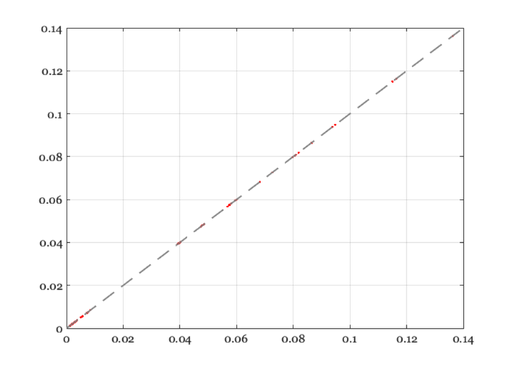
[sensorLinear2, unitSigCurrent2] = sensorCompute(sensorLinear, oi);
sensorLinear2 = sensorSet(sensorLinear2,'name','Linear 2 interp');
% sensorWindow(sensorLinear2);

v2 = sensorGet(sensorLinear2,'volts');
ieNewGraphWin; plot(v1(:),v2(:),'.');
identityLine;

sensorGauss = sensor;
sensorGauss.interp = 'Gauss';
sensorGauss = sensorCompute(sensorGauss, oi);
sensorGauss = sensorSet(sensorGauss,'name','Gaussian interp');
% sensorWindow(sensorGauss);
v3 = sensorGet(sensorGauss,'volts');
ieNewGraphWin; plot(v1(:),v3(:),'.');
identityLine;

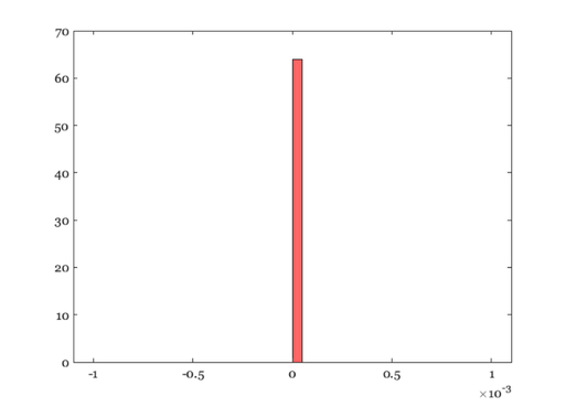
voltsDiff = sensorGet(sensorLinear1, 'volts') - sensorGet(sensorGauss, 'volts');
ieNewGraphWin; imagesc(voltsDiff); colormap(gray(64)); colorbar; axis off;
ieNewGraphWin; histogram(voltsDiff(:), 'BinLimits', [-1e-3, 1e-3], 'BinWidth', 5e-5);

voltsDiffT = unitSigCurrent1 - unitSigCurrent2;
ieNewGraphWin; imagesc(voltsDiffT); colormap(gray(64)); colorbar; axis off;
ieNewGraphWin; histogram(voltsDiffT(:), 'BinLimits', [-1e-3, 1e-3], 'BinWidth', 5e-5);

voltsDiffL = sensorGet(sensorLinear1, 'volts') - sensorGet(sensorLinear2, 'volts');
ieNewGraphWin; imagesc(voltsDiffL); colormap(gray(64)); colorbar; axis off;
ieNewGraphWin; histogram(voltsDiffL(:), 'BinLimits', [-1e-3, 1e-3], 'BinWidth', 5e-5);

ip = ipCreate;

ip = ipCompute(ip, sensorLinear1);
ipWindow(ip);

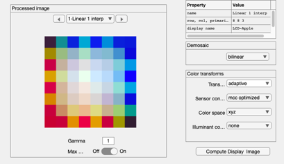
ip = ipCompute(ip, sensorGauss);
ipWindow(ip);