![]()
An Asset class factor model can help make order out of chaos
William F. Sharpe*
This
copyrighted material has been reprinted with permission from The
Journal of Portfolio Management.
Copyright © Institutional Investor, Inc., 488 Madison Avenue,
New York, N.Y. 10022,
a Capital Cities/ABC, Inc. Company. Phone (212) 224-3599.
It is widely agreed that asset allocation accounts for a large part of the variability in the return on a typical investor's portfolio. This is especially true if the overall portfolio is invested in multiple funds, each including a number of securities.
Asset allocation is generally defined as the allocation of an investor's portfolio among a number of "major" asset classes. Clearly such a generalization cannot be made operational without defining such classes.
Once a set of asset classes has been defined, it is important to determine the exposures of each component of an investor's overall portfolio to movements in their returns. Such information can be aggregated to determine the investor's overall effective asset mix. If it does not conform to the desired mix, appropriate alterations can then be made.
Once a procedure for measuring exposures to variations in returns of major asset classes is in place, it is possible to determine how effectively individual fund managers have performed their functions and the extent (if any) to which value has been added through active management. Finally, the effectiveness of the investor's overall asset allocation can be compared with that of one or more benchmark asset mixes.
An effective way to accomplish all these tasks is to use an asset class factor model. After describing the characteristics of such a model, we illustrate applications of a model with twelve asset classes to analyze the performance of a set of open-end mutual funds between 1985 and 1989.
Factor models are common in investment analysis. Equation (1) is a generic representation:
Ri represents the return on asset i, Fi1represents the value of factor 1, Fi2 the value of factor 2, Fin the value of the n'th (last) factor and ei the "non-factor" component of the return on i. All these values are (potentially) unknown before-the-fact, as indicated by the tildes. The remaining values (bi1 through bin) represent the sensitivities of Ri to factors Fi1 through Fin.
A key assumption makes a model of this sort more than simply an exercise in data description: The non-factor return for one asset (ei) is assumed to be uncorrelated with that of every other (e.g. ej). In effect, the factors are the only sources of correlation among returns.
An asset class factor model can be considered a special case of the generic type. In such a model each factor represents the return on an asset class and the sensitivities (bij values) are required to sum to 1 (100%). In effect, the return on an asset i is represented as the return on a portfolio (shown by the sum of the terms in the bracketed expression) invested in the n asset classes plus a residual component (ei). For expository convenience, the sum of the terms in the brackets can be termed the return attributable to style and the residual component (ei) the return due to selection. Indeed, a key contribution of this approach is the separation of return into these two main components.
The usefulness of an asset class factor model depends on the asset classes chosen for its implementation. While not strictly necessary, it is desirable that such asset classes be 1) mutually exclusive, 2) exhaustive and 3) have returns that "differ". Pragmatically, each should represent a market-capitalization weighted portfolio of securities; no security should be included in more than one asset class; as many securities as possible should be included in the chosen asset classe; and the asset class returns should either have low correlations with one another or, in cases in which correlations are high, different standard deviations.
While the appropriate measure of the efficacy of any specific implementation depends on the uses to which the model is to be put, factor models are typically evaluated on the basis of their ability to explain the returns of the assets in question (i.e. the Ris). A useful metric is the proportion of variance "explained" by the selected asset classes. Using the traditional definition, for asset i:
The right-hand side of equation (2) equals 1 minus the proportion of variance "unexplained". The resulting R-squared value thus indicates the proportion of the variance of Ri "explained" by the n asset classes1.
It is important to recognize that this measure indicates only the extent to which a specific model fits the data at hand. A better test of the usefulness of any implementation is its ability to explain performance out-of-sample. For this reason it is important to consider not only the ability of a model to explain a given set of data but also its parsimony. Other things equal (e.g. R-squared values), the fewer the asset classes, the more likely is the model to represent continuing fundamental relationships with predictive content2.
To evaluate the exposures of funds to changes in the returns of key asset classes, the appropriate measure is the collective ability of a set of such classes to explain the time-series variability in the returns on a typical fund (e.g. mutual fund or separately-managed institutional account). Note that this criterion differs from that often applied in evaluating factor models designed to describe specific portions of the overall capital market.
For example, when constructing an equity factor model, one might consider the ability of the selected factors to explain the time-series variation in the returns of a typical stock. Most stock market models include factors representing returns on industry groups and/or economic sectors -- factors that account for much of the typical security's return. If most managers diversify across industries and economic sectors,however, inclusion of factors related to differences in industry and sector returns will add little if any explanatory power to a model designed to explain fund returns.
The model we use has twelve asset classes. The return of each is represented by a market capitalization weighted index of the returns on a large number of securities. For reasons that will become clear, it is important to note that each index represents a strategy that could be followed at low cost using an index fund. The composition of each index is specified in sufficient detail by its provider to enable an investor to track the returns with little error through a passive (index-like) investment strategy.
Table 1 describes the twelve asset classes and the indices used for the associated return series. Most are widely used indexes that require no further description. The four less well-known are those employed to represent U.S. equity classes.
Bills
    Cash-equivalents with less than 3 months to maturity
    Index: Salomon Brothers' 90-day Treasury bill index
Intermediate-term Government Bonds
    Government bonds with less than 10 years to maturity
    Index: Lehman Brothers' Intermediate-term Government Bond Index
Long-term Government Bonds
    Government bonds with more than 10 years to maturity
    Index: Lehman Brothers' Long-term Government Bond Index
 Corporate Bonds
    Corporate bonds with ratings of at least Baa by Moody's or BBB by Standard & Poor's
    Index: Lehman Brothers' Corporate Bond Index
 Mortgage-Related Securities
    Mortgage-backed and related securities
    Index: Lehman Brothers'Mortgage-Backed Securities Index
Large-Capitalization Value Stocks
    Stocks in Standard and Poor's 500-stock index with high book-to-price ratios
    Index: Sharpe/BARRA Value Stock Index
Large-Capitalization Growth Stocks
    Stocks in Standard and Poor's 500-stock index with low book-to-price ratios
    Index: Sharpe/BARRA Growth Stock Index
Medium-Capitalization Stocks
    Stocks in the top 80% of capitalization in the U.S. equity universe after the exclusion
       of stocks in Standard and Poor's 500 stock index
    Index: Sharpe/BARRA Medium Capitalization Stock Index
Small-Capitalization Stocks
    Stocks in the bottom 20% of capitalization in the U.S. equity universe after the exclusion
       of stocks in Standard and Poor's 500 stock index
    Index: Sharpe/BARRA Small Capitalization Stock Index
Non-U.S. Bonds
     Bonds outside the U.S. and Canada
     Index: Salomon Brothers' Non-U.S. Government Bond Index
European Stocks
     European and non-Japanese Pacific Basin stocks
     Index: FTA Euro-Pacific Ex Japan Index
Japanese Stocks
     Japanese Stocks
     Index: FTA Japan Index
In effect, the institutional universe of U.S. equities has been divided into four mutually exclusve and exhaustive groups3. The first two represent a partition of the stocks in Standard and Poor's 500 stock index. Every six months the S&P500 stocks are ranked according to the ratio of the most recently published book value per share to a previous month-end price per share. A dividing line is drawn so that approximately half the total value of the 500 stocks is placed on either side. Stocks with high book-to-price ratios are placed in the "value" stock index; the remainder are in the "growth" stock index.
A similar procedure is followed in constructing the medium capitalization and small capitalization stock indexes. Non-S&P500 stocks are ranked on the basis of total outstanding market capitalization every six months, and a dividing line drawn so that approximately 80% of the total value is above the line and 20% below it. Most of the stocks in the first group are placed in the medium capitalization index and most of the remaining stocks in the small capitalization index. To avoid excessive turnover in the composition of these indexes of relatively illiquid stocks (and an associated high cost for index tracking), any stock that has recently "crossed over the line" a relatively small distance is allowed to remain in its former index4.
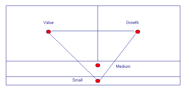
Many of the differences in returns of U.S. equity mutual funds can be attributed to differences in their exposures to these four asset classes. In effect, there appear to be two key dimensions along which such funds differ. One may loosely be termed "value/growth"; the other "small/large". Figure 1 illustrates the composition of the four domestic equity asset classes. Each index can be considered a capitalization-weighted "center of gravity" of the securities in its associated class, as the dots in Figure 1 indicate. Note that any combination of the four indices with non-negative holdings can be represented by a point in the area defined by the index locations (in this case, a triangle)5.
FIGURE 1
COMPOSITION OF FOUR DOMESTIC EQUITY CLASSES
Much has been written about both the small-stock and the value/growth phenomena. While the terms "value" and "growth" reflect common usage in the investment profession, they serve only as convenient names for stocks that tend to be similar in several respects. As is well known, across securities there is significant positive correlation among: book/price, earnings/price, low earnings growth, dividend yield and low return on equity. Moreover, the industry compositions of the value and growth groups differ (e.g. companies with high research budgets tend to have low book values relative to their stock prices).
Those concerned with these distinctions have focused most of their research on long-run average return differences; that is, they have asked whether small stocks or value stocks "do better than they should" in the long-run. Less attention has been paid to likely sources of short-run variability in returns among such groups. For present purposes it suffices that such variability is substantial.
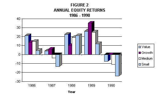
Figure 2 provides relevant evidence: The variability in returns across the four asset classes from year-to-year is far greater than would be encountered if groups with similar numbers of securities had been formed randomly. Fund exposures across these dimensions vary greatly. As a result, much of the variation in fund returns in any given period can be attributed to the combined effects of their exposures to these asset classes and the realized returns on those classes.
The traditional view of asset allocation assumes that an investor allocates assets among (potentially many) funds, each of which holds (potentially many) securities. Ultimately one is interested in the investor's exposures to the key asset classes. These are a function of 1) the amounts of the investor's portfolio invested in the various funds and 2) the exposures of each such fund to the asset classes. The exposures of a fund to the various asset classes are, in turn, a function of 1) the amounts that the fund has invested in various securities and 2) the exposures of the securities to the asset classes.
While it is possible to attempt to determine a fund's exposures from a detailed analysis of the securities held by the fund, a simpler approach typically provides more than enough information for purposes of asset allocation. Such a method uses only realized fund returns to infer the typical exposures of the fund to the asset classes. Since only easily obtained information is required, the approach may be considered "external", in comparison with methods that rely on information that may be available only from sources internal to the fund.
Inspection of equation (1) immediately suggests a procedure that might be used in this connection. Given, say, sixty monthly returns on a fund, along with comparable returns for a selected set of asset classes, one could simply employ a multiple regression analysis with fund returns as the dependent variable and asset class returns as the independent variables. The resulting slope coefficients could then be intererpreted as the fund's historic exposures to the asset class returns.
Table 2 provides an example for Trustees' Commingled U.S. Portfolio (an open-end mutual fund offered by the Vanguard Group). Monthly returns from January 1985 through Decenber 1989 are used for the dependent variable, with the corresponding returns for the twelve asset classes serving as independent variables.
The column entitled "Unconstrained Regression" shows results obtained applying Equation (1). The first twelve rows show the resulting slope coefficients (bij values), expressed as percentages. The coefficient total is shown next, followed by the R-squared value (also expressed as a percentage). A substantial portion (95.20%) of the monthly variance in the fund's returns is explained by this equation. The coefficients, however, do not sum to 100%. What is more important, several are vastly inconsistent with the fund's actual policy (to invest in common stocks with no short positions).
Unconstrained Regression
Constrained Regression Quadratic Programming
The column in Table 2 titled "Constrained Regression" reports the results of a multiple regression analysis similar to the first, with one added constraint: The coefficients were required to sum to 100%. The reduction in R-squared was slight (from 95.20% to 95.16%), but the inconsistency between the coeffficients and the fund's investment policy remains.
The last column in Table 2 reports the results of an analysis where each coefficient is constrained to lie between 0 and 100% and the sum is again required to be 100%. As in the previous cases, the objective of the analysis was to select a set of coefficients that minimizes the "unexplained" variation in returns (i.e., the variance of ei), subject to the stated constraints. An equivalently goal was to maximize the associated value of R-squared, subject to the stated constraints. For this analysis, the presence of inequality constraints ( 0<= bij<= 100% for each i ) required the use of a quadratic programming algorithm.
The addition of constraints reflecting the fund's actual investment policy causes a slight reduction in the fit of the resulting equation to the data at hand (i.e., a decrease in R-squared to 92.22%). Now, however, the coefficients conform far more closely to the reality of the fund's investment style, making the resulting characterization more likely to provide meaningful results with out-of-sample data.
As Table 2 shows, the analysis suggests that the fund traditionally invests so as to obtain returns similar to those achievable with a portfolio with roughly 70% invested in a market-representative portfolio of value stocks and 30% in a market-representative portfolio of small stocks. During the period investigated, over 92% of the month-to-month variation in the return on the fund could be explained by the concurrent variation in the return on this particular mix of value and small stocks.
The use of quadratic programming for the purpose of determining a fund's exposures to changes in the returns of major asset classes is termed style analysis (see Sharpe[1988]). The goal is to find the "best" set of asset class exposures (bij values) that totals to 100% and conforms with rudimentary information concerning the fund's policies (typically, no net short positions in any asset class; for funds known to employ short positions, other bounds may be invoked).. In this context, the best such set of exposures is the one for which the the variance of ei is the least.
Rearranging Equation (1):
The term on the left can be interpreted as the difference between the return on the fund (the first term on the right) and that of a passive portfolio with the same style (shown by sum of the terms in the brackets). The goal of style analysis is to select the style (set of asset class exposures) that minimizes the variance of this difference. Such a difference can be termed the fund's "tracking error" and its variance the fund's "tracking variance".
Note that the objective of such an analysis is not to minimize either the average value of this difference or the sum of the squared differences. Thus the method is not designed to find a style that "makes the fund look bad" (or good). Rather, the goal is to infer as much as possible about the fund's exposures to variations in the returns of the asset classes during the period studied.
We have noted that a quadratic programming algorithm must be used for such an analysis. For an exact solution, one can implement Markowitz' critical line method1(see Markowitz [1987]). This study uses the simpler gradient method described in Sharpe [1987]. Although in principle the latter produces only an approximate solution, differences between the results obtained with the two methods prove to be of no practical importance in this application.
Figure 3 provides a graphical summary of the results shown in the final column of Table 2. The bar chart indicates the estimated style of the fund, and the pie chart the associated R-squared value. In the latter the R-squared value is identified as attributable to the fund's style and the remainder (1 - R-squared) to selection.


It is important to note that the style identified in such an analysis is, in a sense, an average of potentially changing styles over the period covered. Month-to-month deviations of the fund's return from that of style itself can arise from selection of specific securities within one or more asset classes, rotation among asset classes, or both security selection and asset class rotation . For the sake of simplicity, we use the term selection to cover all such sources of tracking differences.
It is sometimes helpful to examine the behavior of a manager's average exposures to asset classes over time. To do so, one can perform a series of style analyses, using a fixed number of months for each analysis through time. Figure 4 shows the results from such a study for Trustee's Commingled U.S. Fund.
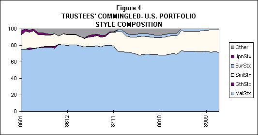
The point at the far right of the diagram represents the style described when the sixty months ending in December 1989 are analyzed. This corresponds to the style shown in Figure 3. Every other point represents the results of an analysis using a different set of sixty monthly returns (note, however, that each such set has fifty-eight months in common with its predecessor). As Figure 4 shows, this fund's style appeared to remain quite constant throughout the period analyzed.
Figures 5 and 6 show the results obtained when the same type of analysis was applied to the returns of Fidelity Magellan Fund -- a highly popular open-end common stock fund. As Figure 5 shows, its style differed considerably from that of Trustees' Commingled U.S. Fund, with emphasis on growth rather than value stocks and exposure to medium-capitalization stocks in addition to smaller ones.
The pie chart in Figure 5 shows that the fund is considerably more diversified (and/or engaged in less rotation) than Trustees' Commingled U.S. Fund. During the period covered, over 97.3% of the monthly variation in Magellan returns could be attributed to the concurrent return on a passive portfolio with the style shown in the bar chart in Figure 5.

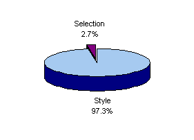
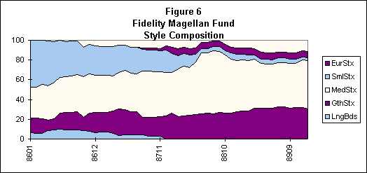
Figure 6 suggests that the Magellan Fund progressively increased its emphasis on large growth stocks and decreased its exposure to small capitalization stocks during the 1980s. This is not surprising, as the fund grew to approximately $14 billion by the end of the period, making substantial investment in very small stocks increasingly difficult.
Figures 3 through 6 show results for two particular mutual funds. Here we provide a more representative view of the efficacy of the procedure, with style analysis performed for each of 395 funds using returns from January 1985 through December 1989. Averages are taken for both the styles and R-squared values of all funds classified as being of the same "type" by Jaye C. Jarrett & Company, Inc., the providers of the data used for this study. In all, seven such types are represented. The results are shown in Figures 7 through 13.
Each figure should be interpreted as representative of the style (bar chart) and variance due to style (pie chart) of a "typical" fund of the type. A portfolio invested in all the funds of a particular type would typically have a much higher R-squared (percent of variance attributable to style) than is shown in the figure in question. Moreover, there is typically considerable variation in both style and R-squared values among the funds within each type group. Given these caveats, the analyses provide useful illustrations of some of the features of the style analysis method.
Figure 7 shows the results for a typical utility stock fund. Such funds (atypically) concentrate their holdings in one industry. As a result, style accounts for an unusally small part (although still 59.3%) of the variance in return. Although such funds hold common stocks, their returns behave more like a passive portfolio invested in both stocks and bonds. That is, utility revenues are "sticky" because to the regulatory process, causing shares of such companies to have features that are both stock-like and bond-like.
The utility fundexample emphasizes the fact that style analysis provides measures that reflect how returns act, rather than a simplistic concept of what the portfolios include. Note, finally, all equity exposure is to value stocks, relflecting the high dividend yields typical of utility shares.


Figure 8 portrays a typical growth equity fund. Here the most prominent exposure is, as expected, to growth stocks, although the typical fund of this type also responds to movements in the returns of other asset classes. Note the exposure to Bills, which probably results from the actual cash holdings that many such funds maintin to meet liquidity needs.
Overall, the results illustrate the fact that few funds are "pure" in the sense of responding only to movements in returns of one asset class. The style analysis procedure can detect some of the subtleties that exist in practice, instead of classifying each fund by a single (pure) style. Finally, note that almost 90% of the monthly variation in return of the typical growth equity fund can be attributed to its style -- a result typical of common stock funds.
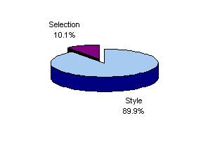
Figure 9 shows the characteristics of a typical growth and income equity fund. Here too, style accounts for approximately 90% of the monthly variation in returns. The effects of a liquidity reserve are probably at least partly responsible for the exposure to Bills, although choices of stocks with lower beta values than those in the asset class indexes could also play a role.
Note the almost perfect balance between value and growth Stocks, relecting an "SP500-like" stance with respect to large-capitalization stocks. The exposures to small and medium stocks may reflect actual investment in such stocks and/or a preference for equal weighting rather than capitalization weighting within the large stock sector. In an important sense, the source of a set of exposures may not even need to be identified, as long as the exposures are representative of likely future results.

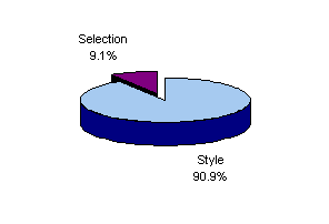
Figure 10 indicates that small stock funds do indeed buy small stocks (as defined by the asset class used for this study). However, they also appear to buy somewhat larger ones. Moreover, there tends to be an emphasis on growth rather than value. This may reflect the actual purchase of large-capitalization growth stocks by some funds. It may also indicate a preference for medium-capitalization stocks with growth characteristics. As Figure 1 suggests, a point lying to the right of the point rerpresentin the medium stock index can be represented by a combination of the large growth stock index, the small stock index and the medium stock index.
As before, the goal is to represent the behavior of the fund, not its precise composition. Finally, note that the R-squared value is slightly lower (87.6%) than for the other diversified funds -- perhaps reflecting the lower liquidity of this sector of the equity market.
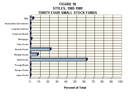
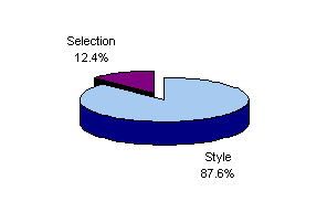
Figure 11 shows that balanced funds are precisely that. While any single fund may diverge substantially from the style shown in the figure, collectively balanced funds provide results similar to those obtained by holding all U.S. asset classes and small amounts of foreign ones. As with other diversified funds, style accounts for roughly 90% of the monthly variation in the returns for the typical fund of this type.
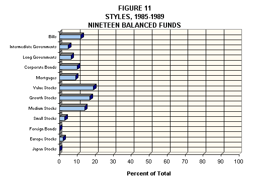
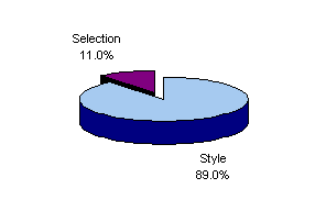
Figure 12 shows that the method works well for bond funds as well as for stock and balanced ones. The typical high-quality bond fund provides exposure to corporate bonds, government bonds and mortgage-related securities, with style accounting for slightly over 88% of monthly variance in return. In any given case, a mix of, e.g., intermediate government bonds and corporate bonds might reflect actual holdings or the average quality of the corporate bond portfolio.
Thus a portfolio with a higher average quality than that reflected in the Corporate Bond Index typically acts more like a mixture of corporate bonds (defined by the index) and intermediate government bonds. Similarly, a portfolio of corporate bonds with a longer duration than that of the Corporate Bond index will "track" more closely with a mix of corporate bonds (defined by the index) and long-term Government bonds. As always behavior, not nomenclature, is relevant.
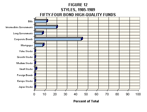

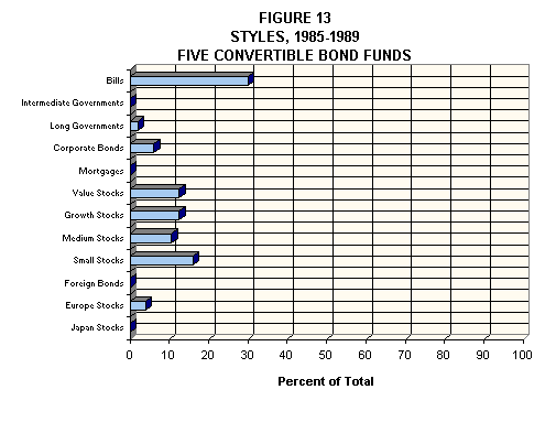
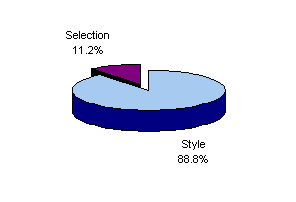
Figure 13 shows a case where an asset class not explicitly represented in a model can be represented well by the classes that are included. As shown, 88.8% of the monthly variation in returns of a typical convertible bond fund can be attributed to the concurrent variation in the returns of a mix of stocks, bills, and bonds. This is not too surprising. A convertible bond has characteristics of both bonds and stocks.
Of course, as bond and stock markets diverge, the relative sensitivities of any given convertible bond to the two markets will change, giving such an instrument its distinctive non-linear characteristic. Interestingly, managers of convertible bond funds appear to have preferred habitats, causing them to buy and sell convertible bonds so as to maintain fairly consistent exposures to asset classes of the type utilized in this study.
As these examples show, a remarkable amount of information can be revealed from an analysis of the returns provided by the manager of an investment fund. This is especially gratifying since in the final analysis return is the product the investor buys from such a manager.
Once the styles of an investor's funds have been estimated, it is a simple matter to determine the associated overall effective asset mix. Letting Wi represent the proportion of the investor's portfolio invested in fund i, overall portfolio return (Rp) will be:
As both equations (1) and (4) are linear, substitution of the former in the latter will provide another linear equation:
or:
where the bpj values are the portfolio's exposures to the asset classes. As can be seen by comparing Equations (5) and (6), each bpj is simply a value-weighted average of the exposures of the component funds to the asset class in question, with the relative amounts invested in the funds used as weights.
The resultant effective asset mix (specified by the values bp1, bp2, ...,bpn ) will account for a large portion of the month-to-month variation in returns for the typical portfolio invested in many funds. Under the assumption that the residual ei terms are uncorrelated, diversification across funds will greatly reduce the variance of the final (non-factor) component and thus increase the portion of variance attributable to asset allocation. Even if some of the residuals are correlated, the use of multiple funds will typically lead to substantial reduction in selection risk.
The effective asset mix represents the style of the investor's overall portfolio. For a multiple-managed portfolio, style is even more important than for an individual fund.
In a sense, a passive fund manager provide an investor with an investment style, while an active manager provides both style and selection. This statements can be used to define the terms "active" and "passive" management. Note that in this taxonomy, the precise implementation of an asset class factor model play a crucial role. This suggests that one may wish to select a set of asset classes so that only superior performance relative to a static mix of the chosen classes warrants the higher fees usually associated with "active" as opposed to "passive" management. This is the approach we take, focusing on a fund's selection return, defined as the difference between the fund's return and that of a passive mix with the same style.
There are several desiderata associated with the selection of a benchmark for performance measurement. A benchmark portfolio should be 1) a viable alternative, 2) not easily beaten, 3) low in cost, and 4) identifiable before the fact.
Style analysis provides a natural method for constructing benchmarks meeting these requirements. The return obtained by a fund in each month can be compared with the return on a mix of asset classes with the same estimated style, where the style is estimated prior to the month in question. Note that this differs from the use of the ei values obtained as byproducts of a style analysis, since the latter are in-sample, not out-of-sample values.
To illustrate the approach for Trustees' Commingled U.S. and Fidelity's Magellan Funds, for each month t:
1. The fund's style is estimated, using returns from months t-60 through t-1.6
2. The return on the resultant style is calculated for month t.
3. The difference between the fund's return in month t and that of the style benchmark determined in steps 1) and 2) is computed. This difference is defined as the fund's Selection Return for month t.
Figure 14 shows the cumulative sum of the monthly selection returns from January 1986 through December 1989 for Trustees' Commingled U.S. Fund.7 In such a graph, increases result from positive selection returns and decreases from negative ones.
.

Average |
-.06 % per month |
Std Dev |
1.69 % per month |
T(Avg) |
-0.25 |
The table below the graph in Figure 14 summarizes the results in a different manner. On average, the fund underperformed its style benchmarks by -0.06% (6 basis points) per month, with a standard deviation of 1.69% (169 basis points) per month. The t-statistic associated with the mean difference was, however, small in absolute value, suggesting that the average difference was not statistically significantly different from zero.8
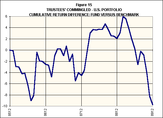
Figure 15 emphasizes the advantages to be gained by analyzing performance the way we have described. It compares the return on Trustees' Commingled U.S. Fund with that of Standard & Poor's 500 stock index (commonly used to evaluate mutual fund performance). The fund's performance, so measured, was over three times as bad as that shown previously: the cumulative difference was -10% and the average difference -20 basis points per month.
But such a comparison includes results due to both style and selection. During the period in question the fund's style underperformed that of the S&P500 (primarily because of its exposure to small stocks). Indeed, this accounts for approximately two-thirds of the fund's underperformance relative to the S&P500.
An investor choosing Trustees' Commingled U.S. Fund could and should have known that its style favored value stocks and small stocks. The choice to expose some of the portfolio to these asset classes should be attributed to the investor. Results (good or bad) associated with such the choice of a style should be attributed to the investor, not to the manager of a fund following that style.
Average |
-.20 % per month |
Std Dev |
2.13 % per month |
T(Avg) |
-0.65 |
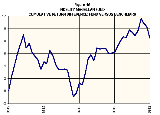
Figures 16 and 17 show the results of similar analyses for Fidelity Magellan Fund. As Figure 16 shows, the fund provided a positive but statistically insignificant outperformance when compared with the S&P500 over the period.
But Figure 17 shows that such a comparison masked Magellan's truly outstanding selection performance. During this period, the fund outperformed its style benchmarks by a cumulative amount of over 25%. Outperformance averaged 57 basis points per month with a standard deviation of 105 basis points. The t-statistic of 3.76 shows that such differences were highly significant statistically. Two aspects account for the large t-value: the relatively large average return difference and the relatively small variation in the difference from month to month.9
Average |
0.18 % per month |
Std Dev |
1.48 % per month |
T(Avg) |
0.84 |
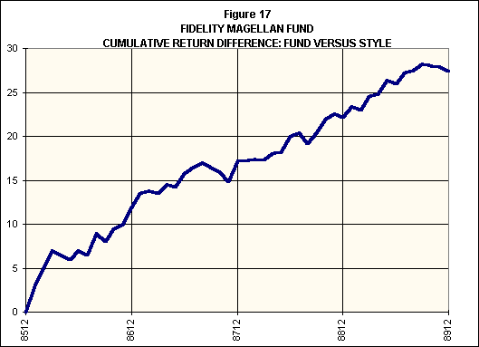
Average |
0.57% per month |
Std Dev |
1.05 % per month |
T(Avg) |
3.76 |
Fidelity Magellan's performance from 1985 through 1989 is far from typical. While only out-of-sample results can provide a definitive test of the collective performance of mutual funds, the average ei values obtained as a by-products from fund style analyses can provide at least some evidence on the matter.
Figure 18 shows the distribution of the average tracking errors obtained from the style analyses of 636 stock, bond and balanced funds. Each value is the average ei value obtained from a style analysis using returns for one fund covering the period from January 1985 through December 1989. Note that the distribution is roughly normal, with a mean of -0.074 (-7.4 basis points per month). This is roughly consistent with the hypothesis that the average mutual fund cannot "beat the market" before costs, because such funds constitute a large (and presumably representative) part of the market. Annualized, the mean underperformance is approximately 0.89% per year -- an amount that, if anything, may be slightly less than the non-transaction costs incurred by a typical mutual fund.
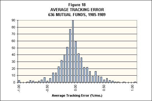
Average = -.074 |
In the paradigm utilized in this article, an investor makes decisions that result in an effective asset mix and a set of selection returns. In a sense, the investor selects a set of (passive or active) managers and a specific allocation of funds among such managers. Given the managers' styles, this determines the investor's effective asset mix.
The procedures described earlier can be applied directly to measure the efficacy with which the investor performs his or her functions. The performance of each month's effective asset mix can be compared with that of a predetermined benchmark asset mix to assess the value added or lost due to asset allocation decisions (advertent or inadvertent). The remainder of the investor's return is attributable to the joint effects of 1) the fund managers' selection returns, and 2) the investor's allocation of money among the managers. The investor selection return (Sp) is simply:
where the Si values are determined out-of-sample, using procedures such as those described earlier.
An asset class factor model can help make order out of the chaos that often attends the investment process. It can provide a consistent view of investment decisions investors make to economize on information flows and exploit comparative advantages. The style analysis procedure described in this article allows such a model to be implemented economically. At the very least it can serve as a valuable supplement to other methods designed to help investors achieve their goals in cost-effective ways.
3. More precisely, BARRA's all-U.S. universe.
5. More generally, the convex hull of the points.
6. For a more operational procedure, returns for a period ending with month t-2 might be used.
7. No compounding is employed in Figure 14 (and the subsequent ones using similar portrayals). This makes it possible to compare vertical distances directly at any point in the figure. Because selection return represents the difference between the returns of two portfolios, compounding would not provide the difference in the cumulative values of the fund and the benchmark. This being said, it should be pointed out that since the logarithm of a monthly value relative will generally differ little from the corresponding monthly return, a graph in which compounded selection returns are shown on a logarithmic scale appears similar to one in which returns are summed and shown on an arithmetic scale, as in this article.
8. The t-statistic is computed by dividing the average return difference by the standard error of the mean (here, the standard deviation of the return difference divided by the square root of 60).
9. The t-statistic is closely related to the reward-to-variability Ratio (sometimes termed the Sharpe Ratio) for the "active" component of a fund's return, which is simply the mean value divided by the standard deviation.
Markowitz, Harry M. Mean-Variance Analyses in Portfolio Choice and Capital Markets. Oxford: Basil Blackwell, Inc. 1987.
Sharpe, William F. "An Algorithm for Portfolio Improvement," in Kenneth D. Lawrence, John B. Guerard, Jr. and Gary D. Reeves, eds. Advances in Mathematical Programming and Financial Planning, Vol. 1, pp. 155-170. Greenwich: JAI Press, Inc., 1987.
---------. "Determining a Fund's Effective Asset Mix," Investment Management Review, December 1988, pp. 59-69.
