Algorithm

We consider linear regression model, where we are given i.i.d. pairs (Y_1,X_1) , (Y_2,X_2) , cdots , (Y_n,X_n) with vectors $X_i in mathbb{R}^p$ and response variables Y_i are given by

Here $theta_0 in mathbb{R}^p$ is the vector of coefficients, W_i is measurement noise with mean zero and variance sigma^2 . Moreover, langle cdot, cdot rangle denotes the standard scalar product in $mathbb{R}^p$ .

In matrix form, letting $Y = (Y_1, cdots, Y_n)^{sf T}$ and denoting by mathbf{X} the design matrix with rows $X_1^{sf T}, cdots, X_n^{sf T}$ , we have

$Y = mathbf{X} theta_0 + W.$

Note: We are primarily interested in high-dimensional regime, where the number of parameters is larger than the number of samples (p > n) , although our method applies to the classical low-dimensional setting (n > p) as well.

Goal

Given response vector and design matrix mathbf{X} , we want to construct confidence intervals for each single coefficient $theta_{0,i}$ .
Furthermore, we are interested in testing individual null hypothesis $H_{0,i} : theta_{0,i} = 0$ versus the alternative $H_{A,i} : theta_{0,i} neq 0$ , and assigning -values for these tests.

Method:

Here, we provide a simple explanation of our method. For more details and discussions, please see our paper.

Our method is based on constructing a ‘de-biased’ version of LASSO.

Let widehat{theta} =widehat{theta}(lambda) be the LASSO estimator with regularization parameter lambda . For a matrix $Min mathbb{R}^{p times p}$ , define

$widehat{theta}^u(M) = widehat{theta} + frac{1}{n} Mmathbf{X}^{sf T}(Y-mathbf{X}widehat{theta}).$

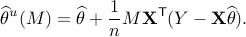
For a suitable choice of matrix , we characterize distribution of the de-biased estimator $widehat{theta}^u$ , from which we construct asymptotically valid confidence intervals, as follows:

For i in {1, cdots, p} and significance alpha in (0, 1) , we let

$J_i(alpha) ,,,, equiv,, [widehat{theta}^u_i - delta(alpha,n), widehat{theta}^u_i + delta(alpha,n)],$
$delta(alpha,n) equiv ,, Phi^{-1}(1-alpha/2) frac{widehat{sigma}}{sqrt{n}} [Mwidehat{Sigma} M^{sf T}]^{1/2}_{i,i}.$

Here, $Phi^{-1}(cdot)$ is the quantile function of the standard normal distribution and widehat{sigma} is a consistent estimator of sigma .

For testing the null hypothesis $H_{0,i}$ , we construct a two-sided -value as follows:

$P_i = 2left(1-Phileft(frac{sqrt{n}|widehat{theta}^u_i|}{widehat{sigma} [Mwidehat{Sigma} M^{sf T}]^{1/2}_{i,i}}right)right).$

How to choose matrix M?

For input parameter , the de-biasing matrix is constructed via the following optimization problem:

1. for i = 1, 2, cdots, p do

Let m_i be a solution of the convex program:

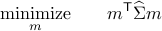
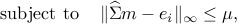
$underset{m}{text{minimize}} quadquad m^{sf T}widehat{Sigma}m$
$text{subject to} quad, |widehat{Sigma} m -e_i|_{infty} le mu,$

where $e_i in mathbb{R}^p$ is the vector with one at the -th position and zero everywhere else.

2. Set 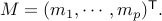$M = (m_1, cdots, m_p)^{sf T}.text{}$ ( Rows of are the vectors m_i .)

In our code, the user can either give parameters lambda and as input or let the algorithm select their values automatically.