In Problem Set One, you got practice with the art of proofwriting in general (as applied to numbers, puzzles, etc.) Problem Set Two introduced first-order logic and gave you some practice writing more intricate proofs than before. Now that we're coming up on Problem Set Three, you’ll be combining these ideas together. Specifically, you’ll be writing a lot of proofs, as before, but those proofs will often be about terms and definitions that are specified rigorously in the language of first-order logic.
The good news is that all the general proofwriting rules and principles you’ve been honing over the first two problem sets still apply. The new skill you’ll need to sharpen for this problem set is determining how to start with a statement like “prove that $f$ is an injection” and to figure out what exactly it is that you’re supposed to be doing. This takes a little practice to get used to, but once you’ve gotten a handle on things we think you’ll find that it’s not nearly as tricky as it might seem.
This page illustrates how to set up proofs of a number of different types of results. While you’re welcome to just steal these proof setups for your own use, we recommend that you focus more on the process by which these templates were developed and the context for determining how to proceed. As you’ll see when we get to Problem Set Four and beyond, you’ll often be given new first-order definitions and asked to prove things about them.
This page is divided into four parts.
- The Big Tables, which explains what you can assume and what you can prove about different first-order logic constructs;
- Proof Templates, which use The Big Tables to show how to structure proofs of definitions specified in first-order logic;
- Defining Things, which explains how to define mathematical objects of different types; and
- Writing Longer Proofs, which explains how to write proofs that feel just a little bit longer than the ones we’ve done so far.
We recommend that during your first read-through here you proceed in order, then flip through the sections in isolation when you need them as a reference.
The Big Tables
As you’ve seen in the past week, we’re starting to use first-order logic as a tool for writing formal definitions, and the structures of the proofs we’ll be writing now depend on how those formal definitions are structured.
Proving Statements
Below is a table of all the first-order logic structures we’ve seen so far, along with what you need to do in order to prove that they’re true. Initially, this table might seem a bit daunting, but trust us – you’ll get the hang of it!
Proving $\forall x. P$
Direct proof: Pick an arbitrary $x$, then prove that $P$ is true for that choice of $x$.
By contradiction: Suppose for the sake of contradiction that there exists some $x$ where $P$ is false. Then derive a contradiction.
Proving $\exists x. P$
Direct proof: Do some exploring and find a choice of $x$ where $P$ is true. Then, write a proof defining $x$ explaining why $P$ is true in that case.
(Proofs by contradiction of existential statements are extremely rare.)
Proving $\lnot P$
Direct proof: Simplify your formula by pushing the negation deeper, then apply the appropriate rule.
By contradiction: Suppose for the sake of contradiction that $P$ is true, then derive a contradiction.
Proving $P \land Q$
Direct proof: Prove each of $P$ and $Q$ independently.
By contradiction: Assume $\lnot P \lor \lnot Q$. Then, try to derive a contradiction.
Proving $P \lor Q$
Direct proof: Prove that $\lnot P \to Q$, or prove that $\lnot Q \to P$. (Great question to ponder: why does this work? You might want to look at the truth tables.)
By contradiction: Assume $\lnot P \land \lnot Q$. Then, try to derive a contradiction.
Proving $P \to Q$
Direct proof: Assume $P$ is true, then prove $Q$.
By contradiction: Assume $P$ is true and $Q$ is false, then derive a contradiction.
By contrapositive: Assume $\lnot Q$, then prove $\lnot P$.
Proving $P \leftrightarrow Q$
Prove both $P \to Q$ and $Q \to P$.
Assuming Statements
Most of the proofs that you’ll write will involve assuming that something is true, then showing what happens as a consequence of those assumptions. The good news is that, like the previous table, there’s a nice set of rules you can use to reason about first-order formulas.
Assuming $\forall x. P$
Initially, do nothing. Do not introduce any variables. Later, should you find some object $z$, you can assume $P$ is true for that choice of $z$.
Important Note: One of the most common mistakes that we see around this point in CS103 is not properly distinguishing between what it means to assume the statement $\forall x. P$ and to prove the statement $\forall x. P$.
If you are proving that $\forall x. P$ is true, you pick an arbitrary $x$ and then try to prove that $P$ is true for that choice of $x$. In other words, you start referring to $x$ as though it’s some concrete thing, then see what happens when you do.
On the other hand, if you assume that $\forall x. P$ is true, you do not make an arbitrary choice of $x$ and prove something about it. Instead, when you make the assumption that $\forall x. P$ is true, just sit tight and wait. As soon as you have some specific $z$ where it would be helpful to know that $P$ were true, you can pull out $\forall x. P$ and conclude that, indeed, $P$ is true for $z$. But simply assuming $\forall x. P$ won’t give you that $x$ to reason about.
Think of a formula of the form $\forall x. P$ as being like a hammer. It says “if you find a nail, you can use this tool to hit the nail.” If I handed you a hammer and said “please hang this picture frame up on the wall,” you wouldn’t start swinging the hammer around hoping that you’d hit a nail somewhere. That would be recklessly dangerous. Instead, you’d say “okay, let me see if I can find a nail.” Then you’d line the nail up where you want it to go, and only then would you swing the hammer at it.
Assuming $\exists x. P$
Introduce a new variable that has property $P$.
When proving an existential statement, you need to do a bunch of work to hunt around and figure out which $x$ will work. But if you’re assuming an existential statement is true, you can immediately say something like “we know there is an $x$ where $P$ is true” and then start using that variable $x$ to refer to that object. A good example is going from “$n$ is even” to “there exists an integer $k$ where $n = 2k$.” You basically get $k$ for free.
Assuming $\lnot P$
Negate $P$, then use this table to see what you’re now assuming.
Assuming $P \land Q$
Assume both that $P$ is true and that $Q$ is true.
Assuming $P \lor Q$
Consider two separate cases, one where $P$ is true and one where $Q$ is true.
Asssuming $P \to Q$
Initially, do nothing. Later, if you find that $P$ is true, you can assume that $Q$ is also true.
Be careful! Like the warning in the section on the universal quantifier, if you are assuming that an implication is true, you should not immediately say something like “assume $P$ is true.” Rather, you should sit back and wait for an opportunity to present itself where $P$ is true.
Assuming $P \leftrightarrow Q$
Assume both $P \to Q$ and $Q \to P$, using the rules above. Or, alternatively, go by cases, one in which you assume both $P$ and $Q$ and one in which you assume both $\lnot P$ and $\lnot Q$.
Proof Template: Bijections
Bijections (functions that are both injective and surjective) are an important and common class of functions with tons of uses. We’ll use them this quarter to talk about cardinality, but they also come up when talking about symmetries, when reasoning about matrix transforms, etc. You are likely to find bijections “in the wild.”
Let’s imagine that you have a function $f : A \to B$ and you want to prove that $f$ is a bijection. How exactly should you go about doing this? As is almost always the case when writing formal proofs, let’s return back to the definition to see what we find. Formally speaking, a function is a bijection if it’s injective and surjective. That means that if we want to prove that $f$ is a a bijection, we’d likely write something like this:
Proof: We will prove that $f$ is injective and surjective.
First, we’ll prove that $f$ is injective. (…)
Next, we’ll prove that $f$ is surjective. (…) ■
Both of those subsequent steps – proving injectivity and surjectivity – is essentially a mini-proof in and of itself.
The above proof template shows how you’d proceed if you found yourself getting to a point in a proof where you needed to show that a particular function is a bijection. There are several different ways that this could happen. First, you might be given a specific function and then be asked to prove something about it. For example, you might come across a problem like this one:
Let $f : \mathbb{R} \to \mathbb{R}$ be the function $f(x) = x^3 + 3x + 1$. Prove that $f$ is a bijection.
In this case, you’ve been handed a concrete function $f$, and the task is to show that it’s a bijection. A proof of this result might look like this:
Proof: We will prove that $f$ is injective and surjective.
First, we’ll prove that $f$ is injective. (…)
Next, we’ll prove that $f$ is surjective. (…) ■
Something to note about the above proof: notice that we didn’t repeat the definition of the function $f$ at the top of the proof before then proceeding to show that $f$ is injective and surjective. This follows a general convention: if you’re proving something about an object that’s explicitly defined somewhere, you should not repeat the definition of that object in the proof. Remember – don’t restate definitions; use them instead (see the Discrete Structures Proofwriting Checklist for more information).
As a great exercise, go and fill in the blank spots in the above proof!
On the other hand, you might be asked to show that an arbitrary function meeting some criteria is also a bijection. We did an example of this in lecture:
Prove that if $f : A \to A$ is an involution, then $f$ is a bijection.
In this case, we should structure our proof like this:
Proof: Pick an arbitrary involution $f : A \to A$. We will prove that $f$ is injective and surjective.
First, we’ll prove that $f$ is injective. (…)
Next, we’ll prove that $f$ is surjective. (…) ■
Notice that in this case, we had to explicitly introduce what the function $f$ is, since we’re trying to prove a universally-quantified statement (“if $f$ is an involution, then …”) and there isn’t a concrete choice of $f$ lying around for us to use.
Proof Template: Injectivity
Suppose you have a function $f : A \to A$. To prove that $f$ is injective, you need to show that
\[\textcolor{blue}{\forall x_1 \in A. \forall x_2 \in A.} (\textcolor{red}{f(x_1) = f(x_2)} \to \textcolor{purple}{x_1 = x_2}) \text.\]Remember our first guiding principle: if you want to prove that a statement is true and that statement is specified in first-order logic, look at the structure of that statement to see how to structure the proof. So let’s look at the above formula. From the structure of this formula, we can see that
- the reader picks arbitrary elements $x_1$ and $x_2$ from A (since these variables are universally-quantified);
- we assume that $f(x_1) = f(x_2)$ (since that’s the antecedent of an implication); and then
- we want to show that $x_1 = x_2$ is true (since it’s the consequent of an implication).
This means that a proof of injectivity will likely start off like this:
Consider some arbitrary $x_1, x_2 \in A$ where $f(x_1) = f(x_2)$. We want to show that $x_1 = x_2$. (…)
At this point, the structure of the proof will depend on how $f$ is defined. If you have a concrete definition of $f$ lying around, you would likely go about expanding out that definition. For example, consider the function $f : \mathbb{R} \to \mathbb{R}$ defined as
\[f(x) = 42x + 137\text.\]Suppose we wanted to prove that $f$ is injective. To do so, we might write something like this:
Proof: Consider some arbitrary real numbers $x_1$ and $x_2$ where $f(x_1) = f(x_2)$. We want to show that $x_1 = x_2$. To see this, note that since $f(x_1) = f(x_2)$, we have $42x_1 + 137 = 42x_2 + 137$. (…)
Notice that we did not repeat the definition of the function $f$ in this proof. The convention is that if you have some object that’s explicitly defined outside of a proof (as $f$ is defined here), then you don’t need to – and in fact, shouldn’t – redefine it inside the proof. Also, although the definition of injectivity is given in first-order logic, note that there is no first-order logic notation in this proof: no connectives, no quantifiers, etc. Just plain English. (I mean, I guess technically functions are something we see in first-order logic, but that’s a different use of functions than what we’re doing here.)
Alternatively, it might be the case that you don’t actually have a concrete definition of $f$ lying around and only know that $f$ happens to satisfy some other properties. For example, let’s return to the definition of involutions that we introduced in lecture. As a reminder, a function $f : A \to A$ is called an involution if the following is true:
\[\forall a \in A. f(f(a)) = a\text.\]So let’s imagine that we know that $f$ is an involution (and possibly satisfies some other properties) and we want to show that $f$ is injective. In that case, rather than expanding the definition of $f$ (since we don’t have one), we might go about applying the existing rules we have. That might look like this, for example:
(…) Consider some arbitrary $x_1, x_2 \in A$ where $f(x_1) = f(x_2)$. We want to show that $x_1 = x_2$. To see this, note that since $f(x_1) = f(x_2)$, we know that $f(f(x_1)) = f(f(x_2))$. Then, since $f$ is an involution, we see that $x_1 = x_2$, as required. (…)
Notice how we invoked the fact that f was an involution: we didn’t write out the general definition of an involution and then argue that it applies here. Instead we just said how we could use the statements we began with, plus the definition of an involution, to learn something new.
There is one other detail about proving injectivity that we need to discuss. As we mentioned in lecture, there are two equivalent ways of defining what it means for a function $f : A \to B$ to be injective. We discussed one of them above. Here's the other:
\[\textcolor{blue}{\forall x_1 \in A. \forall x_2 \in A.} (\textcolor{red}{x_1 \ne x_2} \to \textcolor{purple}{f(x_1) \ne f(x_2)})\text.\]If we want to use this definition in a proof, then we
- have the reader picks arbitrary elements $x_1$ and $x_2$ from A (since these variables are universally-quantified);
- we assume that $x_1 \ne x_2$ (since that’s the antecedent of an implication); and then
- we want to show that $f(x_1) \ne f(x_2)$ is true (since it’s the consequent of an implication).
For example, we might write a proof like this:
Consider some arbitrary $x_1, x_2 \in A$ where $x_1 \ne x_2$. We want to show that $f(x_1) \ne f(x_2)$. (…)
If you use this template, all the same rules apply from above. If $f$ is already given to you as a concrete object, then don’t repeat its definition in the proof. If you’re proving a result of the form “any function of type $X$ is an injection,” make sure to first tell the reader to pick some function of type $X$ before you try proving it’s an injection. And make sure to not use quantifiers, connectives, etc. in your proof.
Proof Template: Not Injective
In the previous example, we saw how to prove that a function does have some particular property. What happens if you want to show that a function does not have some particular property?
For example, let’s suppose $f : A \to B$ is a function and we want to prove that $f$ is not injective. How do we do this? The good news is that, because we have a first-order logic definition for injectivity, we can simply negate that definition to show that something is not injective. Specifically, we’re interested in the negation of this statement:
\[\forall x_1 \in A. \forall x_2 \in A. (x_1 \ne x_2 \to f(x_1) \ne f(x_2)\text.\]Here's the negation:
\[\textcolor{blue}{\exists x_1 \in A. \exists x_2 \in A.} (\textcolor{red}{x_1 \ne x_2 \land f(x_1) = f(x_2)})\text.\]We can now read off the negation to see what it’s asking us to prove. If we want to show that a function is not injective, then
- we pick specific $x_1 \in A$ and $x_2 \in A$ (because these variables are existentially-quantified), then
- we need to show that $x_1 \ne x_2$ and that $f(x_1) = f(x_2)$ (because that’s the statement being quantified).
Notice that the use of the existential quantifier here changes up the dynamic of the proof. We don’t say “hey reader, give me whatever values you’d like” and then proceed from there. That’s what we’d do if these variables were universally-quantified. Instead, we have to go on a scavenger hunt to find concrete choices of $x_1$ and $x_2$ that make the quantified statement true.
There are many ways you could write up a proof of this form. For example, you could write something like this:
Let $x_1 = \blank$ and $x_2 = \blank$. We need to show that $x_1 \ne x_2$ and that $f(x_1) = f(x_2)$. (…)
We need to show that a certain $x_1$ and $x_2$ exist satisfying some criteria, so we just say what choices we’re going to make and justify why those choices are good ones. The specific justification is going to depend on the particulars of what we know about $f$. If $f$ is a specific, concretely-chosen function, we can just plug in values of $f$ to see that everything above checks out. If, on the other hand, $f$ is an arbitrarily-chosen function with certain auxiliary properties, then we’ll need to appeal to those particular properties to get the result we want.
The hard part of writing a proof like this is probably going to be coming up with what choices of objects you’re going to pick in the first place rather than writing down your reasoning. As with all existentially-quantified proofs, be prepared to draw out a bunch of pictures, to try out some concrete examples, etc.
Proof Template: Surjectivity
Let’s suppose you have a function $f : A \to B$. If you want to prove that $f$ is surjective, you need to prove that the following statement is true:
\[\textcolor{blue}{\forall b \in B.}\textcolor{red}{\exists a \in A.}\textcolor{purple}{f(a) = b}\text.\]Following the general rule of “match the proof to the first-order definition,” this means that in our proof,
- the reader picks an arbitrary element $b$ from $B$ (since this variable is universally-quantified</a>), then
- we pick a specific $a \in A$ that meets the requirements (since this variable is existentially-quantified</a>), and finally we
- we prove that $f(a) = b$ is true (since it’s the statement that’s being quantified).
Notice how this statement is a mix of a universally-quantified statement and an existentially-quantified statement. This means that one step of the proof is to ask the reader to pick $b$ outside our control, and another is to then think long and hard about how to choose a specific $a$ to get the desired effect.
As a result, a proof of surjectivity will often start off with this:
Pick any $b \in A$. Now, let $a = \blank$. We need to show that $f(a) = b$.
As before, the next steps in this proof are going to depend entirely about what we know about the function $f$. If we have a concrete definition of $f$ in hand (say, if the proof is taking an existing function that we’ve defined and then showing that it’s surjective), then we’d need to look at the definition of $f$ to see what to do next.
Alternatively, it might be the case that you don’t actually have a concrete definition of $f$ lying around and only know that $f$ happens to satisfy some other properties. In that case, you’d have to use what you knew about the function $f$ in order to establish that $f(a) = b$.
Proof Template Exercises: Other Types of Proofs
In the preceding sections, we went over some examples of how you’d structure proofs of different properties of functions. However, we didn’t cover all the different properties you might want to consider. That’s intentional – ultimately, it’s more important that you understand how to look at a first-order statement and determine what it is that you need to prove than it is to approach these problems as an exercise in pattern-matching.
Here are a few exercises that you may want to work through as a way of seeing whether you’ve internalized the concepts from this handout.
-
A function $f : A \to A$ is called an involution if the following is true:
\[\forall a \in A. f(f(a)) = a\text.\]Write a proof template for showing that a function $f$ is an involution.
-
A function $f : A \to A$ is called idempotent if the following is true:
\[\forall a \in A. f(f(a)) = f(a) \text.\]Write a proof template for showing that a function $f$ is idempotent.
-
A function $f : A → A$ has a fixed point if the following is true:
\[\exists a \in A. f(a) = a\text.\]Write a proof template for showing that a function $f$ has a fixed point.
-
A function $f : A \to B$ is called doubly covered if the following is true:
\[\forall b \in B. \exists a_1 \in A. \exists a_2 \in A. \left( a_1 \ne a_2 \land f(a_1) = f(a_2) = b \right) \text.\]Write a proof template for showing that a function $f$ is doubly-covered.
Defining Functions
In the course of writing a proof, you may need to give a concrete example of a function with a particular property. As you saw in lecture, there are a few ways to define a function. In all cases, you should be sure to do the following:
- Give the domain and codomain.
- Give a rule explaining how to evaluate the function.
- Confirm that it obeys the domain/codomain rules.
Here’s an example of what this might look like. Suppose we want to define a function that takes in a natural number, outputs a natural number, and works by adding one to its argument. Here’s one way to do just that:
Consider the function $f : \mathbb{N} \to \mathbb{N}$ defined as $f(n) = n + 1$. To confirm this is indeed a function, pick some $n \in \mathbb{N}$; we'll show that $f(n) \in \mathbb{N}$. Notice that $f(n) = n + 1$ is a natural number, as needed.
Notice how we have all the necessary pieces here. We give the domain and codomain using the normal syntax ($f : \mathbb{N} \to \mathbb{N}$), we give a rule for the function ($f(n) = n + 1$), and we check that each natural number (element of the domain) maps to a natural number (element of the codomain).
Sometimes you can define functions with simple rules, where the function is some mathematical expression. Sometimes, you’ll need to define functions with more complex rules, where how the function behaves depends on some property of the input. For that, you can use a piecewise function. Here’s an example of what that might look like:
Consider the function $f : \mathbb{Z} \to \mathbb{Z} defined as follows:
\[f(x) = \left\lbrace \begin{aligned} x^2 & \text{if } x \lt 0 \\ x^3 & \text{if } x \ge 0 \end{aligned} \right.\]To quickly confirm that $f$ is a valid function, pick any $x \in \mathbb{Z}$; we'll show that $f(x) \in \mathbb{Z}$ as well. If $x \lt 0$, we see that $f(x) = x^2$, and $x^2$ is an integer. Otherwise, we have $x \ge 0$ and $f(x) = x^3$ is an integer.
If you do define a piecewise function, much like when you’re writing a proof by cases, the written proof doesn’t require you to exhaustively confirm that all cases are covered, but you absolutely should do this on your own to ensure you didn’t miss anything!
Another way to define a function is to take some existing functions and combine them together. In that case, you don’t need to give an explicit rule. For example, suppose that you already have two functions $f : A \to B$ and $g : B \to C$ lying around. Then you could do something like this:
Let $h = g \circ f$.
At this point, no further elaboration is necessary. The composition operator $\circ$ is well-known and indeed produces a legal function given two input functions whose domain and codomain agree with one another, so there’s no need to explain why $h$ obeys the domain/codomain rule. (Stated differently – it’s not that there was no need to check that $h$ obeyed these rules, but rather that we already did that outside the proof when defining composition and no further elaboration is needed.) And we don't need to state the domain and codomain of $h$ here, since that can be inferred from $f$ and $g$.
The last way you can define a function is by drawing pictures showing the domain and codomain and how the function is evaluated. This will only work on functions whose domain and codomain are finite – you can’t draw infinitely many items in a picture – and is most common when you’re trying to show that it’s possible for some function to have some particular property. Here's an example of this:
Consider the function $f : A \to B$ defined below:
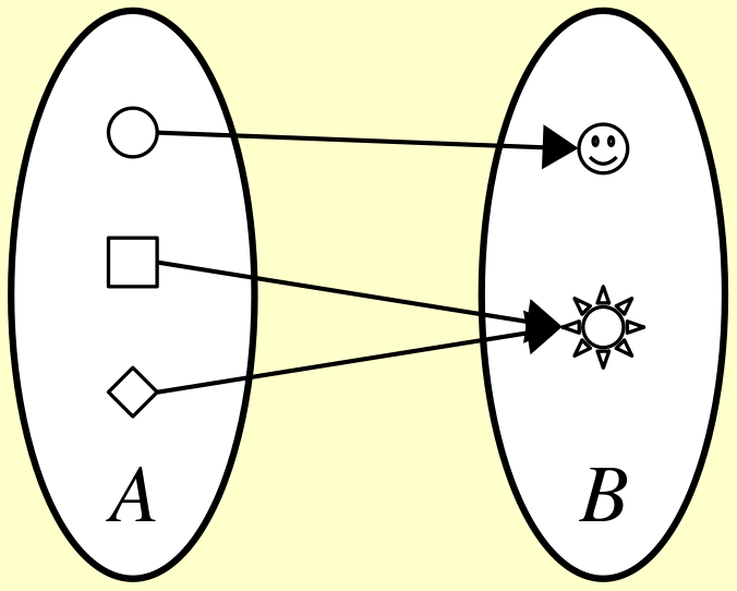
Here, the reader can see what the sets $A$ and $B$ are and what the rule is for evaluating the function $f$. This is another exception to the normal rule that you have to validate the domain/codomain rule, since in the case of a function the expectation is “hey reader, I assume you’ve checked there’s exactly one arrow coming out of everything in $A$, and I’m not going to explain this to you.” 😃
Writing Longer Proofs
You might find, in the course of writing up proofs on discrete structures, that you need to prove several connected but independent results. For example, if you’re proving a function is a bijection, then you need to prove that it’s both injective and surjective. Sometimes, that fits comfortably into a single proof. But, just as it’s good advice to break longer pieces of code into multiple helper functions, it’s sometimes easier to write a longer proof by breaking it down into multiple smaller pieces.
This is where lemmas come in. A lemma is a smaller proof that helps establish a larger result. The distinction between a lemma and a theorem is purely one of context. Usually, a theorem is the big overall result you’re trying to establish, and a lemma is just a small result that helps build into it.
Lemmas come in many forms. Sometimes, they’re smaller proofs of technical results needed to establish the main theorem, but which are less “exciting” or “neat” than the main result. Sometimes, they’re simply smaller fragments of a bigger result, especially one that has multiple parts.
Here’s an example of a proof broken up into lemmas. (All the terms and definitions mentioned are completely fictitious.)
Lemma 1: For all whagfis $x$, if $x$ is gammiferous, then $x$ is haoqi-complete.
Proof: (some kind of proof goes here). ■
Lemma 2: Let $Q$ be an o’a’aa. Then $Q$ is a syththony.
Proof: (some kind of proof goes here). ■
Theorem: Every ichenochen is a zichenzochen.
Proof: Consider an arbitrary ichenochen $J$. We need to show that $J$ is zichenzochen.
Pick any gammiferous whagfi $q$ that cowarbles with $J$. By Lemma 1, we know that $q$ is haoqi-complete. By Gloomenberg’s Theorem, we know that $q$ is an o’a’aa, so by Lemma 2 we know that $q$ is a syththony. And since $J$ is an ichenochen with a cowarbling syththony, we know that $J$ is zichenzochen, as required. ■
Silly terms aside, the basic pattern here is the following. We state and prove two lemmas that we’ll use later in the theorem. Then, in the body of the theorem, we refer back to those lemmas to establish the results we need to establish. That keeps the body of the theorem’s proof short and offloads the complexity elsewhere.