Sentaurus Workbench
2. Running Projects

2.1 Opening Sentaurus Workbench Projects
2.2 Understanding Node Colors
2.3 Cleaning Up Project Directories
2.4 Running Projects
2.5 Selecting Nodes
2.6 Displaying Node Information
2.7 Viewing Output Results
2.8 Deleting Projects
2.9 Overview of Files Associated with Sentaurus Workbench Simulation Nodes

Objectives

• To run a Sentaurus Workbench project.

2.1 Opening Sentaurus Workbench Projects

For this part of the module, the project SWB_nmos will be used. It is located in the directory Applications_Library/GettingStarted/SWB_nmos. Locate and select this project in the projects browser. Then, select Edit > Copy (Ctrl+C) and Edit > Paste (Ctrl+V) to copy the project under the $STDB directory or a subdirectory of it.

Then, double-click the copy of the project under $STDB. This opens the project and it appears in the right pane of the main window (see Figure 1).

Figure 1. Main window of Sentaurus Workbench showing tool flow (black border), parameters (blue border), and simulation tree (red border). (Click image for full-size view.)

The tool flow refers to the sequence of simulation tools and their associated input files. In the SWB_nmos example, these are Sentaurus Process, Sentaurus Structure Editor, Sentaurus Device, and Inspect as seen in Figure 1. Below the tool flow, the project parameters (Type, Igate, and so on) and the corresponding simulation nodes ([n1], [n2], and so on) are listed.

To display node numbers: View > Tree Options > Show Node Numbers (or press the F9 key).

A complete sequence of simulation nodes (comprising all tools in the tool flow) form an experiment. In other words, an experiment is a complete horizontal line in the table view. Any number of experiments is possible for a given tool flow if parameters are used.

To the right of the tool flow, there are variables and electrical extracted parameters from the simulated I_d–V_d characteristics: Vtgm, Vti, Id, SS, gm, Lgeff, Xj, Ygox, Tox (use the scroll bar to see them all). When the simulation is completed, the electrical extracted values appear in their respective columns.

2.2 Understanding Node Colors

Every simulation node in a project has a color associated with it that indicates its status. The color chart in the lower-right corner of the main window of Sentaurus Workbench (see Figure 2) shows what each color indicates.

Figure 2. Colors indicating different node statuses.

For example, when the project SWB_nmos is opened, the nodes are yellow, indicating that the nodes were simulated previously, and blue, which gives some information about the process and device steps. This is because a (successfully run) project was copied from the Applications_Library.

The format in which the Sentaurus Workbench project tree is displayed is very flexible and user controllable. You can display solely the tool flow, or the number the various simulation nodes, or display parameters (splits), variables, extracted values, and other details.

To use this feature:

• From the View menu, select or clear the various options, or View > Tree Options for more features.

2.3 Cleaning Up Project Directories

Before running this project (SWB_nmos) from the beginning, clean up the project results from the previous run.

To clean up a project:

1. Project > Clean Up (Ctrl+L).
2. In the Cleanup Options dialog box, select the items to be removed (see Figure 3).
3. Click OK.

Figure 3. Cleanup Options dialog box.

Sentaurus Workbench deletes all files associated with the previous run, and the project is now ready to run. This is indicated by a change in the color of the nodes from yellow (done) to white (none).

2.4 Running Projects

To run a project:

1. Project > Run (Ctrl+R) or click the corresponding toolbar button ().
   The Run Project dialog box is displayed (see Figure 4), which is used to select which nodes to run (all unsimulated nodes by default) as well as which simulation queue to use (running on the local host is the default).
2. Click Run to start the simulation.

Figure 4. Run Project dialog box.

Sentaurus Workbench proceeds to run the project, and the Project Log dialog box is displayed (see Figure 5) with real-time updates on the status of the project.

Figure 5. Project Log dialog box. (Click image for full-size view.)

As the simulation runs, the nodes change status from "none" (white) to "queued" (light green) to "pending" (bright green) to "running" (blue) and finally to "done" (yellow). If a node fails, it becomes "failed" (red).

To stop a running simulation:

• Nodes > Abort (Ctrl+T) or click the corresponding toolbar button ().

After the project run is completed, all variables are extracted (Vtgm, Vti, and Id) and displayed to the right of the tool flow in the main window of Sentaurus Workbench.

2.5 Selecting Nodes

Instead of entering which nodes to run in the Run Project dialog box, the nodes that need to run can be selected in the table (hold the Ctrl key to select multiple nodes), before clicking the Run button. For example, to run only the Sentaurus Process nodes associated with HaloEnergy=25, select nodes 10 and 13, and then click the Run button.

Figure 6. Selecting nodes in table. (Click image for full-size view.)

If you want to run an entire experiment (row), click the row number. Multiple rows can be selected as well.

To select all nodes to the right of a certain node, in other words, to run all nodes starting with a particular one, click that node and use Nodes > Extend Selection To > Leaves. Similarly, all nodes that need to be completed before a particular node can be run are selected using Nodes > Extend Selection To > Root. Other node selection criteria can be found in Nodes > Select.

2.6 Displaying Node Information

To find the properties of any node, double-click the respective node. The Node Explorer is displayed (see Figure 7).

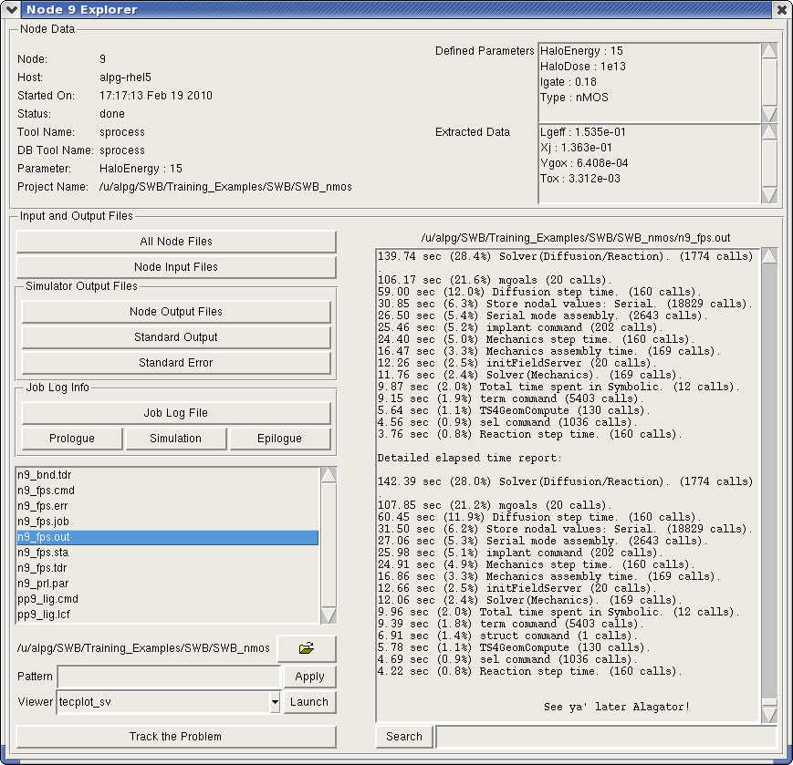
Figure 7. Node Explorer for node 9. (Click image for full-size view.)

The Node Explorer displays the following information

• Node number.
• The computer on which the simulation was performed.
• Date and time of the simulation.
• Node status.
• Corresponding tool (Sentaurus Process in Figure 7).
• Corresponding parameter (HaloEnergy) with its value.
• Project directory.

The Node Explorer also displays all input and output parameters associated with the node on the left part.

The bottom part of the Node Explorer displays all files associated with the node. These can be categorized using the buttons on the left, or individual files can be selected using the file list. Text files can be viewed in the file viewer on the right.

2.7 Viewing Output Results

A given node has several input and output files associated with it. These can be viewed by right-clicking a node and selecting Visualize. All text and log files can be viewed using the text editor SEdit by selecting them.

All output data files in the case of Sentaurus Process, Sentaurus Device, and Sentaurus Device Electromagnetic Wave Solver can be viewed using Tecplot SV, or a plot of .plx and .plt files in Sentaurus Device can be viewed using Inspect.

In addition, the information written to standard output, when a simulation is running, can be viewed by selecting Nodes > View Output (Ctrl+W).

An alternative method of viewing output is to click the toolbar button.

2.8 Deleting Projects

To delete the project SWB_nmos:

1. Select the project in the projects browser.
2. Right-click and select Delete.

If an error message is displayed (see Figure 8), it means that the project must be closed before deleting it.

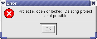
Figure 8. Error message dialog box.

In this case, click OK, and select Project > Close. (The project disappears from the main window.)

Now, repeat Steps 1–2, and click Yes in the dialog box that is displayed.

2.9 Overview of Files Associated with Sentaurus Workbench Simulation Nodes

Master input files (that is, the input files that users write and that, in general, contain variables) are named <tool_label>_<tool_acronym>.cmd. For each tool, there is a default tool_label that is assigned to a tool instance. You can specify your own tool_label in the Tool Properties dialog box. The name tool_acronym is assigned automatically to the generic input file.

Table 1 lists the most commonly used tools, their default tool label, and tool acronym.

Table 1. Tools, default tool labels, and tool acronyms used in Sentaurus Workbench.

Tool	Default tool label	Tool acronym
Sentaurus Process	sprocess	fps
Sentaurus Topography	sptopo, sptopo3d	tpg, t3d
Sentaurus Interconnect	sinterconnect	sis
Sentaurus Structure Editor	sde	dvs
Ligament Flow Editor	–	lig*
Ligament Layout Editor	–	prl*
Sentaurus Mesh	snmesh	msh
Noffset3D	noffset3d	pof
Sentaurus Device	sdevice	des
Sentaurus Device Monte Carlo	smoca	moc
Sentaurus Band Structure	sband	epm**
Sentaurus Device Electromagnetic Wave Solver	emw	eml
Inspect	inspect	ins
Tecplot	tecplot	tec
Sentaurus Data Explorer	tdx	tdx**
shell	cshell	csh
tclsh	gtclsh	tcl
my tool	mytool	myt

* Ligament Flow Editor and Ligament Layout Editor are not used as separate tool instances. Their tool label is determined from the calling tool. For example, if Ligament Flow Editor is used with Sentaurus Process, the tool label is fps.
** Sentaurus Band Structure and Sentaurus Data Explorer use input files with the extension .tcl.

The master input files with their default tool labels are, therefore, sprocess_fps.cmd, sdevice_des.cmd, and so on. If there is more than one instance of the same tool, a number is added to the default tool label.

A simulation project is launched in two steps:

• First, the Sentaurus Workbench preprocessor generates parameterized input files from the generic input files. This means that, for each value a variable or parameter can assume, a unique simulator input file is generated.
• Second, for each unique simulator input, the appropriate simulator is launched.

The simulator is launched using the batch tool gjob, which produces two output files per simulation node: n@node@_<tool_acronym>.job and n@node@_sge.err. Information about the preprocessing of a project can be found in the file preprocessor.log. The simulator output files are named n@node@_<tool_acronym>.<extension> and pp@node@_<tool_acronym>.<extension>. For example, all files n3_fps.<extension> belong to Sentaurus Workbench node number 3 that performs a process simulation with Sentaurus Process.

Table 2 lists the most commonly generated files belonging to simulation nodes. These are the files that are listed in Sentaurus Workbench with the Node Explorer.

Table 2. File name extensions in a Sentaurus Workbench project.

File name extension	Description	Remarks
cmd	Preprocessed simulation input command file.	Sentaurus Workbench variables are replaced by their actual values.
err	File containing simulator error messages.	Error messages generated by Tcl procedures or licensing can be found here as well.
sge.err	Error messages from gjob.	Contains error messages from gsub if the job failed.
out, log	Simulation log file.	Information about the progress of the simulation.
plt	Device simulation current file.	Contains solution variables at device terminals (such as voltages and currents).
sta	Status of the simulation.	The status can be one of the following: none | queued | running | failed | aborted | done. The status is indicated by the color of the simulation node, which also contains information about the execution host.
tdr	The structure with simulation results.	Contains field data such as doping distribution and electrostatic potential.
job	Information from gjob.	Contains information from the preprocessor and the simulation job submission. Watch here for error messages if a simulation node is not executed.
par	Preprocessed parameter file.	Used in Sentaurus Device, EMW, and Ligament Layout Editor.

For some extensions, there can be more than one file, depending on the simulation task. Additional files are written by the simulators if users specify them in the simulator input file.