Quadrature rules
GUIDING QUESTION:
How can I compute an integral numerically?
Motivation
The definite integral
$$\int_a^b f(x) dx$$
computes the area under the graph of $f$, between $x = a$ and
$x = b$.
How can I compute it?
The
Riemann integral
is defined as a limit of Riemann sums
Riemann sum.
Guiding philosophy: We may approximate this limit numerically by taking a finite sum.
Quadrature rules
So we set out to find nodes $x_0, x_1, \ldots, x_n \in [a, b]$ and
weights $w_0, w_1, \ldots, w_n$ to approximate
$$\int_a^b f(x) dx \color{var(--emphColor)}{\approx} \displaystyle \sum_j w_j f_j,$$
with $f_j = f(x_j)$.
Déjà vu?
$$f'(x_i) \approx \sum_j \alpha_j f_j$$
In the
last module,
we used linear combinations of function values to approximate
the function's derivative.
Here, we'll find which linear combinations of function values
are good approximations to the function's
definite integral!
Via interpolant
We'll
also use the interpolating polynomial
here.
Let $x_0, x_1, \ldots, x_n$ denote $\bbox[3pt, border: 3pt solid var(--emphColor)]{n + 1}$
evenly-spaced nodes on the interval $[a, b]$.
Let $p(x)$ denote the polynomial of degree
at most $n$ interpolating $f$ at the given $x_i$.
We'll approximate
\begin{equation*}
\int_a^b f(x) dx \color{var(--emphColor)}{\approx} \int_a^b p(x) dx.
\end{equation*}
We'll restrict our attention to equidistant nodes for
simplicity.
Newton-Cotes quadrature
The nodes are given, so we need only find the right weights $\color{var(--emphColor)}{w_j}$.
We'll obtain these by integrating the interpolating polynomial $p$
analytically.
Newton-Cotes quadrature
In the
Lagrange basis,
$p(x) = \sum_j f_j L_j(x)$, so
\begin{align*}
\int_a^b f(x) dx &\approx \int_a^b p(x) dx = \int_a^b \sum_{j = 0}^n f_j L_{j}(x) dx \\
\end{align*}
\begin{align}
& \,\,= \sum_{j = 0}^n \bigg( \int_a^b L_{j}(x)dx \bigg) f_j \\
& \,\,= \displaystyle \sum_j \color{var(--emphColor)}{w_j} f_j,
\end{align}
with $\color{var(--emphColor)}{w_j} = \int_a^b L_j(x) dx$.
When deriving finite difference formulas, we
obtained
\begin{equation*}
f'(x_i) \approx p'(x_i) = \sum_{j = 0}^n \color{var(--emphColor)}{d_{ij}} f_j,
\end{equation*}
with $\color{var(--emphColor)}{d_{ij}} = L_{j}'(x_i)$.
We have an analogous statement here!
\begin{equation*}
\int_{a}^{b} f(x) dx \approx \int_a^b p(x) dx = \sum_{j = 0}^n \color{var(--emphColor)}{w_j} f_j,
\end{equation*}
with $\color{var(--emphColor)}{w_j} = \int_{a}^{b} L_{j}(x) dx$.
When computing derivatives or integrals numerically, we approximate
the desired quantity by a weighted sum
of function values, and performing the appropriate operation on the
Lagrange basis polynomials gives the right weight.
When the nodes $x_j$ are given and the weights $\color{var(--emphColor)}{w_j}$
are defined by
integrals of Lagrange basis polynomials, the quadrature rule
$$\int_a^b f(x) dx {\approx} \displaystyle \sum_j \color{var(--emphColor)}{w_j} f_j$$
is a Newton-Cotes (NC) rule.
The rule is said to be closed if
$x_0 = a$ and $x_n = b$.
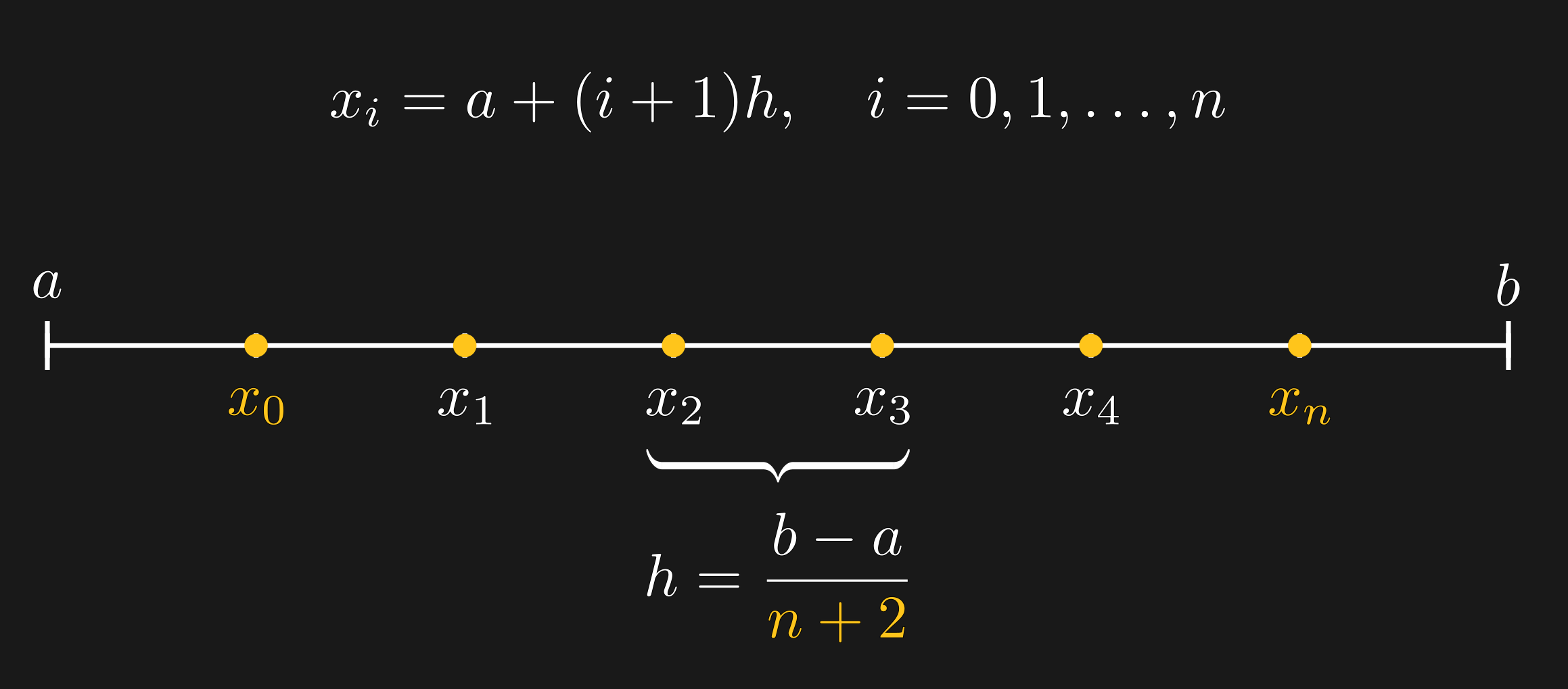
Otherwise, the rule is said to be open.
Since we are considering equidistant nodes only, the nodes for a
closed rule are
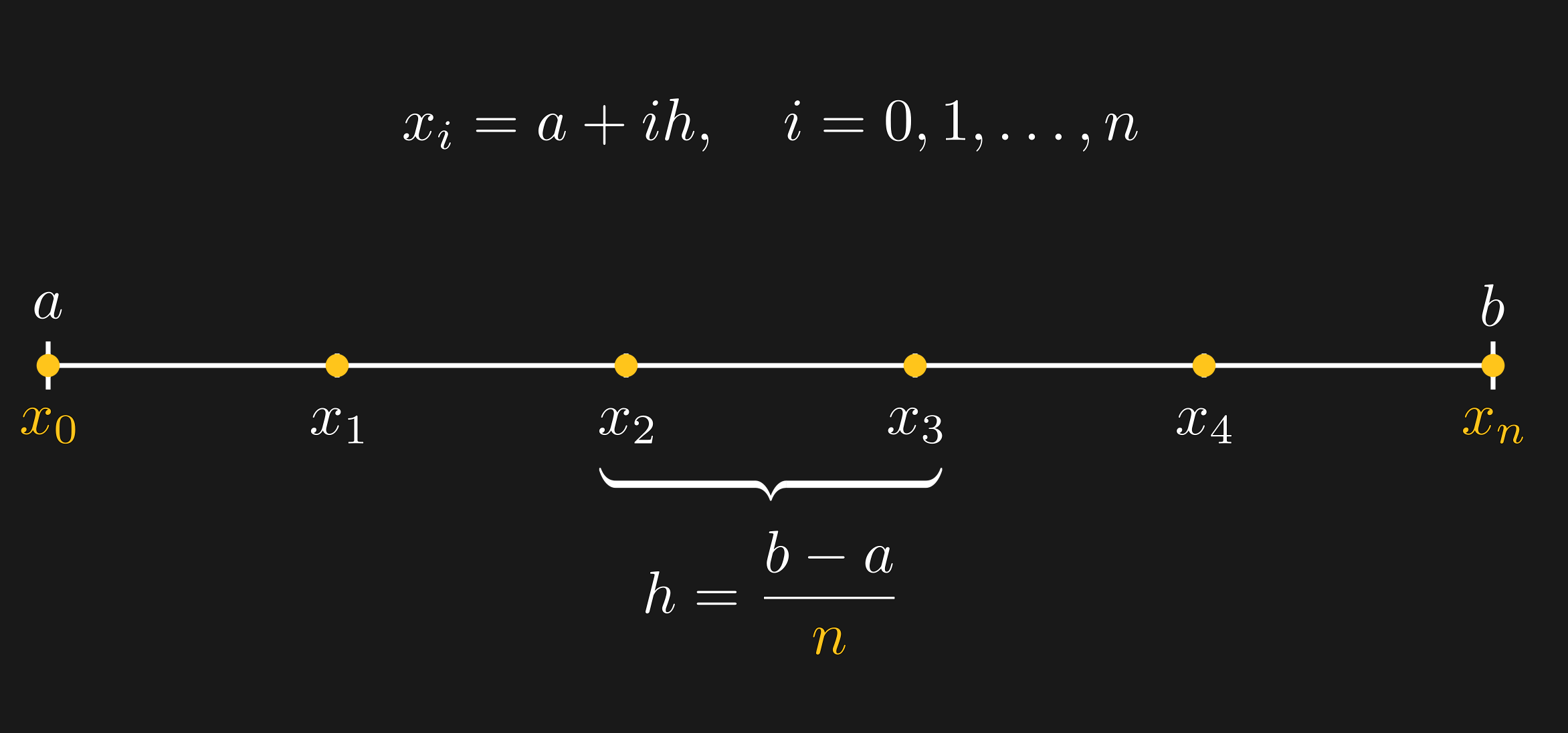
When the rule is open, the nodes are
General Newton-Cotes
To specify an NC rule, we must
- Decide whether it is open or closed
- Determine $\bbox[3pt, border: 3pt solid var(--emphColor)]{n + 1}$, the number of nodes
- Compute $w_j = \int_a^b L_{n,j}(x)dx$, where $L_{j}$ denotes the $j$th Lagrange basis polynomial.
(Closed NC rule, $\bbox[3pt, border: 3pt solid var(--emphColor)]{n + 1} = 3$)
As usual, let $h = x_{i+1} - x_i$. The rule is closed, so
$x_0 = a$, $x_1 = (a + b)/2$, $x_2 = b$, and $h = (b-a) / 2$.
By definition,
$$\color{var(--emphColor)}{w_0} = \int_a^b L_{0}(x) dx
= \int_a^b \frac{(x-x_1)(x-x_2)}{(x_0-x_1)(x_0 - x_2)} dx.$$
The substitution $$\bbox[3pt, border: 3pt solid var(--emphColor)]{x = a + th}$$ is very helpful when computing the weights!
(Closed NC rule, $\bbox[3pt, border: 3pt solid var(--emphColor)]{n + 1} = 3$)
The rule is closed, so $h = x_{i+1} - x_i = (b-a) / 2$ and
therefore
$$x_0 = a, \quad x_1 = (a + b)/2, \quad \text{and} \quad x_2 = b.$$
By definition,
$$\color{var(--emphColor)}{w_0} = \frac{h}{2} \int_0^2 (t-1)(t-2) dt$$
(Closed NC rule, $\bbox[3pt, border: 3pt solid var(--emphColor)]{n + 1} = 3$)
The rule is closed, so $h = x_{i+1} - x_i = (b-a) / 2$ and
therefore
$$x_0 = a, \quad x_1 = (a + b)/2, \quad \text{and} \quad x_2 = b.$$
By definition,
$$\color{var(--emphColor)}{w_0} = \frac{h}{2} \bigg(\frac{t^3}{3} - \frac{3}{2}t^2 + 2t \bigg|_{t=2}\bigg)$$
(Closed NC rule, $\bbox[3pt, border: 3pt solid var(--emphColor)]{n + 1} = 3$)
The rule is closed, so $h = x_{i+1} - x_i = (b-a) / 2$ and
therefore
$$x_0 = a, \quad x_1 = (a + b)/2, \quad \text{and} \quad x_2 = b.$$
By definition,
$$\color{var(--emphColor)}{w_0} = \frac{h}{3}$$
(Closed NC rule, $\bbox[3pt, border: 3pt solid var(--emphColor)]{n + 1} = 3$)
The rule is closed, so $h = x_{i+1} - x_i = (b-a) / 2$ and
therefore
$$x_0 = a, \quad x_1 = (a + b)/2, \quad \text{and} \quad x_2 = b.$$